2. Chapter 2. FLO-2D Model Theory

FLO-2D is a simple volume conservation model. It moves the flood volume around on a series of tiles for overland flow or through stream segments for channel routing. Floodwave progression over the flow domain is controlled by topography and resistance to flow. Flood routing in two dimensions is accomplished through a numerical integration of the equations of motion and the conservation of fluid volume for either a water flood or a hyperconcentrated sediment flow. A discussion of the governing equations follows.

2.1. Governing Equations

The constitutive fluid motion equations include the continuity equation and the momentum equation:

(2.1)\[ \frac{\partial h}{\partial t} + \frac{\partial hV}{\partial x} = i\]

(2.2)\[ S_f = S_o - \frac{\partial h}{\partial x} - \frac{V}{g} \frac{\partial V}{\partial x} - \frac{1}{g} \frac{\partial V}{\partial t}\]

where:

h is the flow depth

V is the depth-averaged velocity in one of the eight flow directions x.

i is the excess rainfall intensity; and may be nonzero on the flow surface.

S_f is the friction slope component; and is based on Manning’s equation.

S_o is the bed slope pressure gradient

The other terms include convective and local acceleration terms.

This equation represents the one-dimensional depth averaged channel flow. For the floodplain, while FLO-2D is multi-direction flow model, the equations of motion in FLO-2D are applied by computing the average flow velocity across a grid element boundary one direction at time. There are eight potential flow directions, the four compass directions (north, east, south and west) and the four diagonal directions (northeast, southeast, southwest and northwest). Each velocity computation is one-dimensional and is solved independently of the other seven directions. Since the flow is being shared with all of a given grid element neighbors, resolution of the velocity vectors is not required. The stability of this explicit numerical scheme is based on strict criteria to control the magnitude of the variable computational timestep. The equations representing hyperconcentrated sediment flow are discussed later in the manual.

Understanding the relative magnitude of the acceleration components to the bed slope and pressure terms is important. Henderson (1966) computed the relative magnitude of momentum equation terms for a moderately steep alluvial channel and a fast-rising hydrograph as follows:

	Bed Slope	Pressure Gradient	Convective Acceleration	Local Acceleration
Momentum Equation Term:	So	∂h/∂x	V∂V/g∂x	∂V/g∂t
Magnitude (ft/mi)	26	0.5	0.12 - 0.25	0.05

This illustrates that the application of the kinematic wave (S_o = S_f) on moderately steep slopes with relatively steady, uniform flow is sufficient to model floodwave progression and the contribution of the pressure gradient and the acceleration terms can be neglected. The addition of the pressure gradient term to create the diffusive wave equation will enhance overland flow simulation with complex topography. The diffusive wave equation with the pressure gradient is required to predict floodwave attenuation and the change in storage on the floodplain. The local and convective acceleration terms in the full dynamic wave equation are important to the flood routing for flat or adverse slopes or very steep slopes or unsteady flow conditions. Only the full dynamic wave equation is applied in FLO-2D model and the contribution of each term in the equation is computed regardless of an assumption of negligibility.

2.2. Solution Algorithm - How the Model Works

The differential form of the continuity and momentum equations in the FLO-2D model is solved with a central, finite difference numerical scheme. This explicit algorithm solves the momentum equation for the flow velocity across the grid element boundary one element at a time. The solution to the differential form of the continuity and momentum equations results from a discrete representation of the equation when applied at a single point. Explicit schemes are simple to formulate but usually are limited to small timesteps by strict numerical stability criteria. Finite difference schemes can require lengthy computer runs to simulate steep rising or very slow rising floodwaves, channels with highly variable cross sections, abrupt changes in slope, split flow and ponded flow areas.

The FLO-2D computational domain is discretized into uniform, square grid elements. The computational procedure for overland flow involves calculating the discharge across each of the boundaries in the eight potential flow directions (Figure 4) and begins with a linear estimate of the flow depth at the grid element boundary. The estimated boundary flow depth is an average of the flow depths in the two grid elements that will be sharing discharge in one of the eight directions. Non-linear estimates of the boundary depth were attempted in previous versions of the model, but they did not significantly improve the results. Other hydraulic parameters are also averaged between the two grid elements to compute the flow velocity including flow resistance (Manning’s n-value), flow area, slope, water surface elevation and wetted perimeter. The flow velocity (dependent variable) across the boundary is computed from the solution of the momentum equation (discussed below). Using the average flow area between two elements, the discharge for each timestep is determined by multiplying the velocity times flow area.

The full dynamic wave equation is a second order, non-linear, partial differential equation. To solve the equation for the flow velocity at a grid element boundary, initially the flow velocity is calculated with the diffusive wave equation using the average water surface slope (bed slope plus pressure head gradient). This velocity is then used as a first estimate (or a seed) in the second order Newton-Raphson tangent method to determine the roots of the full dynamic wave equation (James, et. al., 1977). Manning’s equation is applied to compute the friction slope. If the Newton-Raphson solution fails to converge after 3 iterations, the algorithm defaults to the diffusive wave solution.

In the full dynamic wave momentum equation, the local acceleration term is the difference in the velocity for the given flow direction over the previous timestep. The convective acceleration term is evaluated as the difference in the flow velocity across the grid element from the previous timestep. For example, the local acceleration term (1/g*∂V/∂t) for grid element 251 in the east (2) direction converts to:

(2.3)\[\frac{\Delta \left( V_{t} - V_{t-1} \right)_{251}}{g \cdot \Delta t}\]

where:

V_t is the velocity in the east direction for grid element 251 at time t,

V_t-1 is the velocity at the previous timestep (t-1) in the east direction,

∆t is the timestep in seconds,

g is the acceleration due to gravity.A similar construct for the convective acceleration term (V_x/g*∂V/∂x) can be made where V₂ is the velocity in the east direction and V₄ is the velocity in the west direction for grid element 251:

(2.4)\[V_2 \cdot \frac{\Delta \left( V_2 - V_4 \right)_{251}}{g \cdot \Delta x}\]

The discharge across the grid element boundary is computed by multiplying the velocity times the cross sectional flow area. After the discharge is computed for all eight directions, the net change in discharge (sum of the discharge in the eight flow directions) in or out of the grid element is multiplied by the timestep to determine the net change in the grid element water volume. This net change in volume is then divided by the available surface area (A_surf = storage area) on the grid element to obtain the increase or decrease in flow depth ∆h for the timestep.

(2.5)\[\sum Q_x^{i+1} = Q_n + Q_e + Q_s + Q_w + Q_{ne} + Q_{se} + Q_{sw} + Q_{nw} = A_{surf} \frac{\Delta h}{\Delta t}\]

where:

Q_x = discharge across one boundary

A_surf = surface area of one grid element

∆h/∆t = change in flow depth in a grid element during one timestep

The channel routing integration is performed in the same manner except that the flow depth is a function of the channel cross section geometry and there are usually only one upstream and one downstream channel grid element for sharing discharge. The computational index is the flow direction (1 of 8 directions) not the grid element. This simplifies and reduces the number of steps in the solution algorithm. Each direction is visited only once during a sweep of the grid system domain and involves two grid elements whereas a grid element index requires each grid element to be visited (Figure 4).

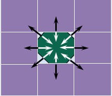
Figure 4. Flow Direction.

Flow Direction is the Computational Index not the Grid Element Number. To summarize, the solution algorithm incorporates the following steps:

For a given flow direction location in the grid system, the average flow geometry, roughness and slope between two grid elements are computed.

The flow depth d_x for computing the velocity across a grid boundary for the next timestep (i+1) is estimated from the previous timestep i using a linear estimate (the average depth between two elements).

(2.6)\[d_x^{i+1} = d_x^i + d_{x+1}^i\]

The flow direction first velocity overland, 1-D channel or street estimate is computed using the diffusive wave equation. The only unknown diffusive wave equation variable is the velocity.

The predicted diffusive wave velocity for the current timestep is used as a seed in the Newton-Raphson method to solve the full dynamic wave equation for the velocity. It should be noted that for hyperconcentrated sediment flows such as mud and debris flows, the velocity calculations include the additional viscous and yield stress terms.

The discharge Q across the boundary is computed by multiplying the velocity by the cross sectional flow area. For overland flow, the flow width is adjusted by the width reduction factors (WRFs).

The incremental discharge for the timestep across the eight boundaries (or upstream and downstream channel elements) are summed:

(2.7)\[\Delta Q_x^{i+1} = Q_n + Q_e + Q_s + Q_w + Q_{ne} + Q_{se} + Q_{sw} + Q_{nw}\]

and the change in volume (net discharge x timestep) is distributed over the available storage area within the grid or channel element to determine an incremental increase in the flow depth.

(2.8)\[\Delta d_x^{i+1} = \Delta Q_x^{i+1} \, \Delta t / A_{surf}\]

where:

ΔQ_x is the net change in discharge in the eight floodplain directions for the grid element for the timestep Δt between time i and i + 1. See Figure 5.

The numerical stability criteria are then checked for the new flow depth. If the Courant number stability criteria is exceeded, the timestep is reduced to the Courant number computed timestep, all the previous timestep computations are discarded and the velocity computations begin again with the first computational flow direction.

The simulation progresses with increasing timesteps using a timestep algorithm until the stability criteria are exceeded again.

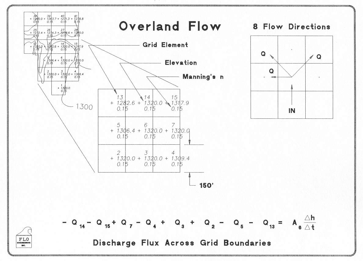
Figure 5. Discharge Flux across Grid Element Boundaries.

To accomplish the discharge exchange between grid elements based on the flow direction, the model sets up an array of side connections at runtime as shown in Figure 6. These flow directions are only accessed once during a timestep instead of the dual visitation required by searching for contiguous elements. This approach facilitates additional parallel processing for model speedup and has the additional benefits of:

• Reducing the required discharge computations by about 40% increasing model speed.

• Ignoring completely blocked sides.

• Eliminating NOFLOC assignment for channels.

In this computation sequence, the grid system inflow discharge and rainfall are computed first, and then the channel flow is computed. Next, if streets are being simulated, the street discharge is computed and finally, overland flow in 8-directions is determined (Figure 6). After all the flow routing for these components has been completed, the numerical stability criteria are tested for every floodplain, channel or street element. If stability criteria of any element are exceeded, the timestep is reduced by various functions depending on the previous history of stability success and the computation sequence is restarted. If all the numerical stability criteria are successfully met, the timestep is increased for the next grid system computational sweep. During a sweep of the grid system for a timestep, discharge flux is added to the inflow elements, flow velocity and discharge between grid elements are computed and the change in storage volume in each grid element for both water and sediment are determined. All the inflow volume, outflow volume, change in storage or loss from the grid system area are summed at the end of each time step and the volume conservation is computed. Results are written to the output files or to the screen at user specified output time intervals.

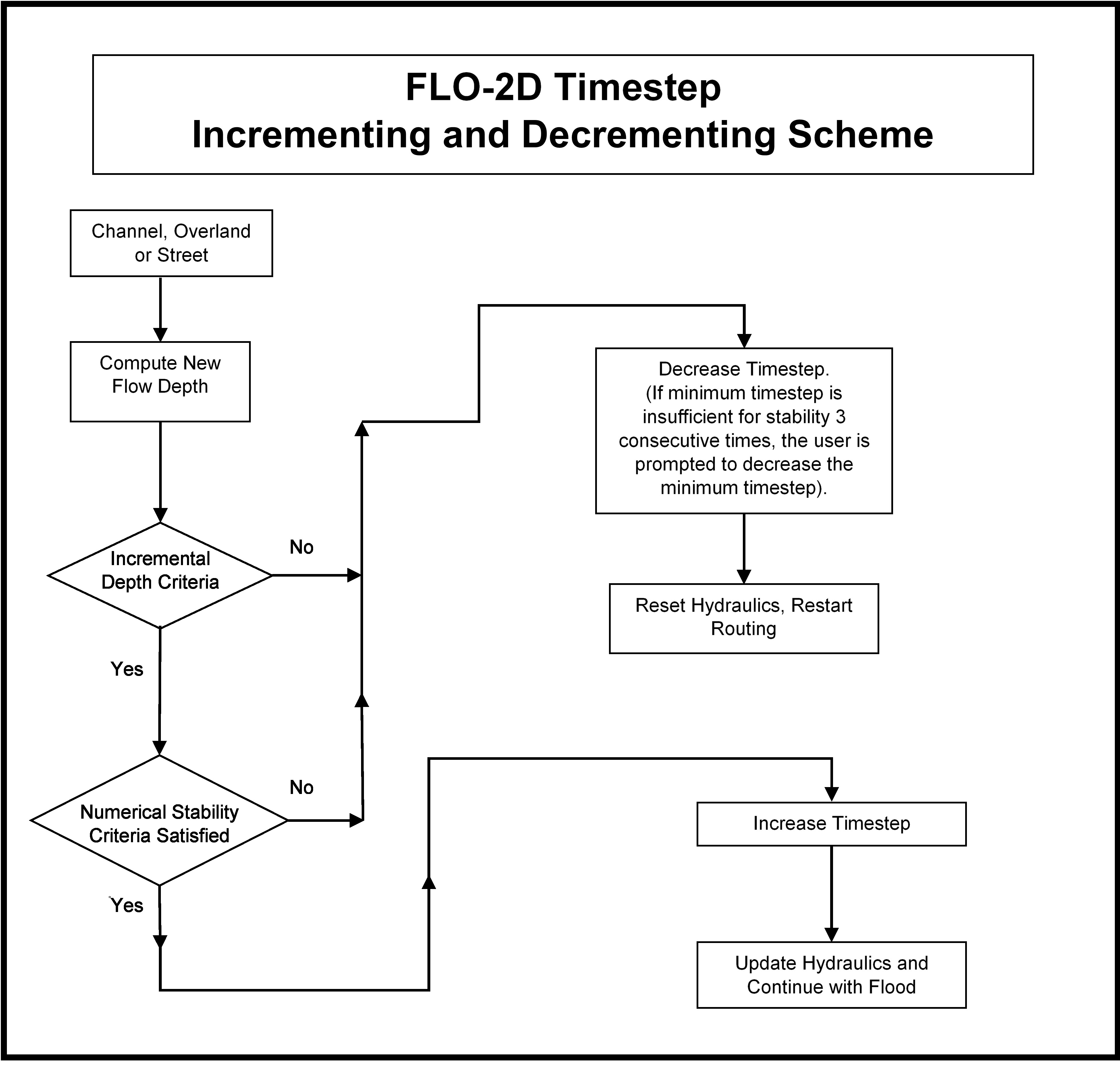
Figure 6. FLO-2D Stability Criteria Flow Chart.

The FLO-2D flood routing scheme proceeds on the basis that the timestep is sufficiently small to ensure numerical stability (i.e. no numerical surging). The key to efficient finite difference flood routing is that numerical stability criteria limits the timestep to avoid numerical surging and yet allows large enough timesteps to complete the simulation in a reasonable time. FLO-2D has a variable timestep depending on whether the numerical stability criteria are exceeded. The numerical stability criteria are checked for every grid element at every timestep to ensure that the solution is stable. If the numerical stability criteria are exceeded, the timestep is decreased and all the previous hydraulic computations for that timestep are discarded. Most explicit schemes are subject to the Courant-Friedrich-Lewy (CFL) condition for numerical stability (Jin and Fread, 1997). The CFL condition relates the floodwave celerity to the model time and spatial increments. The physical interpretation of the CFL condition is that a particle of fluid should not travel more than one spatial increment Δx (grid element side) in one timestep Δt (Fletcher, 1990). FLO-2D uses the CFL condition for the floodplain, channel and street routing. The timestep Δt is limited by:

(2.9)\[\Delta t = \frac{C \, \Delta x}{\beta V + c}\]

where:

C is the Courant number (C ≤ 1.0)

Δx is the square grid element width or channel length

V is the computed average cross section velocity

β is a coefficient (5/3 for a wide channel)

c is the computed wave celerity

While the coefficient C can vary from 0.2 to 1.0 depending on the type of explicit routing algorithm, a default value of 0.6 is recommended in the FLO-2D model. When C is set to 1.0, artificial or numerical diffusivity is theoretically zero for a linear convective equation (Fletcher, 1990). If the simulation has some numerical surging identified by unreasonably high velocities or spikes in an outflow discharge hydrograph, the Courant number should be reduced by 0.1 until a value of 0.2 or 0.3 is reached. The Courant number is spatially variable by grid element within a small range. With successful completion the cell Courant number is permitted to increase by 0.0001 up to a value 0.05 greater than the assigned value. If the Courant number is exceeded, the value is decreased by 0.002 until the assigned value is reached. The assigned Courant is the minimum value allowed.

It may not be possible to completely avoid artificial diffusivity or numerical dispersion using the Courant number to limit the timestep (Fletcher, 1990). Timesteps range from 0.1 second to 30 seconds with a typical timestep on the order of 1 second during the highest discharge flux. The model starts with a minimum timestep equal to 5 seconds and increases it until the numerical stability criteria exceeded, then the timestep is reset to the computed Courant number timestep. If the stability criteria continue to be exceeded, and the minimum timestep is not small enough to conserve volume or maintain numerical stability, then the input data must be modified. The timesteps are a function of the discharge flux for a given grid element and its size. Small grid elements with a steep rising hydrograph and large peak discharge require small timesteps. Accuracy is not compromised if small timesteps are used, but the runtime time can be long if the grid system is large.

The timestep incrementing and decrementing functions were designed to support the role of the Courant number in the model stability. It was determined that varying the Courant number within a certain range of the original value reduced the number of ineffective timestep decreases. In addition, the timestep increments and decrements were reduced to enable the computational timestep to adjust to numerical stability criteria more gradually. This replaced the method of a large timestep decrease followed by more numerous small timestep increases. Results show there was a significant increase in runtime model speed up from 15 to 40%. The stability criteria are applied as follows:

• Separate Courant number assignment for floodplain, channel and street flow.

• Automated spatial variation in the floodplain, channel or street Courant number within a specified range depending on the whether the Courant number criteria was exceeded or not exceeded.

It should be noted that the obsolete stability parameters DEPTOL (% change in flow depth) and WAVEMAX (dynamic wave) stability criteria has been eliminated.

A timestep accelerator parameter (TIME_ACCEL) was coded into the model. Several adjustments to this variable have been made over the years. The default value was changed from 0.1 to 1.0. A higher value of TIME_ACCEL will result in larger timestep increments. When the computational timestep is less than 1.0 second and a simulation timestep loop was successfully completed without exceeding the stability criteria, the timestep is incremented by the TIME_ACCEL (default 1.0) + 0.001. If the timestep was 0.5, then the next timestep would be increased to 0.501 seconds. If the timestep is greater than 1 second, then the timestep increment is:

(2.10)\[\text{DSEC} = \text{DSEC} + \frac{\text{TIME_ACCEL} \cdot 0.0085}{\text{XFAST}}\]

where:

DSEC = computational timestep in seconds

TIME_ACCEL = Coefficient to increase the rate of incremental timestep change. Default value = 0.1. A value of 0.1 may result in a more stable simulation time. A value of 0.2 or higher may result in a faster simulation.

XFAST = XFAST + 0.001 for each successfully completed timestep loop when DSEC > 1.0 second. Resets to 1.0 each time the DSEC timestep is decremented.

This algorithm increases the timestep uniformly until the timestep DSEC is greater than 1 second. When DSEC > 1.0, successive increases in DSEC result in a larger value of XFAST which begins to slow down the timestep rate of change. The maximum timestep is limited to 30 seconds.

2.3. The Importance of Volume Conservation

A review of any flood model simulation results begins with volume conservation. Volume conservation indicates accuracy and numerical stability. The inflow volume, outflow volume, changes in storage and losses (infiltration) are summed at the end of each time step. FLO-2D volume conservation results are written to the output files or to the screen at user specified output time intervals. Data errors, numerical instability, or poorly integrated components may cause a loss of volume conservation. Any simulation not conserving volume should be revised. It should be noted that volume conservation in any flood simulation is not exact. While some numerical error is introduced by rounding numbers, approximations, or interpolations (such as with rating tables), volume should be conserved within a fraction of a percent of the inflow volume. The user must decide on an acceptable level of error in the volume conservation. While volume conservation with 0.001 percent is considered very accurate, most FLO-2D simulations have a volume conservation accuracy within a few millionths of one percent.

2.4. Courant Number Variability for Numerical Stability

The key to efficient FLO-2D flood routing is assigning numerical stability criteria that limits the timestep to avoid surging and yet allows large enough timesteps for a fast simulation. FLO-2D has a variable timestep that is a function of the numerical stability criteria. The numerical stability criteria are checked for every grid element flow direction for each timestep. If any of the numerical stability criteria are exceeded, the timestep is decreased and all the previous hydraulic computations for that timestep are discarded.

The FLO-2D computation routing algorithm is an explicit scheme that is subject to the Courant-Friedrich-Lewy (CFL or Courant number) condition for numerical stability. The Courant number relates the floodwave movement to the model discretization in time and space. The concept of the Courant number is that a particle of fluid should not travel more than one spatial increment Δx (between the center of cells) in one timestep Δt. If the model computational timestep exceeds the Courant relationship timestep, the stability criteria is exceeded and a timestep decrement occurs. Mathematically the Courant relationship is given by:

(2.11)\[V + c = \frac{C \, \Delta x}{\Delta t}\]

where:

C = Courant Number (C ≤ 1.0)

Δx = FLO-2D square grid element width (distance between node centers)

V = depth averaged velocity

c = floodwave celerity = (gd)^0.5, where;

g is gravitation acceleration.

d is the flow depth above the thalweg.

This equation relates the progression of the floodwave (V + c) to the discretized model in space and time. The Courant number C can vary from 0.1 to 1.0, and a value of 1.0 will enable the model to have the largest possible timestep. When C is set to 1.0, artificial or numerical diffusivity is theoretically zero for a linear convective equation. Testing has shown that the FLO-2D model can run faster (more consistent higher timesteps) with greater stability if the Courant number is set to values less than 1.0. The FLO-2D default Courant number is 0.6 which will provide a numerically stable model for most applications. Rearranging the CFL relationship, the model computes the Courant timestep Δt as:

(2.12)\[\Delta t = \frac{C \, \Delta x}{V + c}\]

Numerical instability occurs when the computational timestep is too large or the rate of change in the timestep is too large and too much volume enters or leaves a grid element (discharge flux). The corresponding change in flow depth can result in a high velocity (or Froude number) with the discharge causing a rapid fluctuation in the grid element water surface elevation (surging). Numerical surging may cause spikes in the discharge hydrograph (Figure 7), adverse water surface slope in the downstream direction or unreasonable maximum velocities (VELTIMEFP.OUT (Figure 8) for the floodplain or VELTIMC.OUT for channels) or Froude numbers (SUPER.OUT). Unreasonable maximum velocities are easy to identify because the VELTIM_x.OUT files are sorted in descending order. The first several reported maximum velocities should not be significantly greater than the rest of the file as in the case of node 4887 in the VELTIMFP.OUT file below.

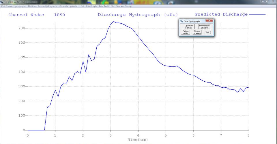
Figure 7. Numerical Surging in a Channel Element Hydrograph.

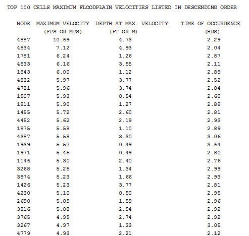
Figure 8. File Sample VELTIMFP.OUT.

Using the Courant Number and Timestep Accelerator Parameter

The global Courant Number is assigned in the TOLER.DAT file line 2 as follows:

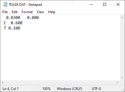
Figure 9. File Sample TOLER.DAT.

where C is a line character identifier and the Courant number for floodplain, channel and street are entered. The Courant number should only be assigned for those components that are used. The channel and street components may not be used in a given project.

The typical range of the Courant number is from 0.2 (slower more stable model) to 0.9 (faster less stable model). The default of 0.6 is recommended as a starting value. For models that appear to be unstable, reducing the Courant Number to a lower value in decrements of 0.1 (from 0.6 to 0.5 down to 0.2) should control any numerical surging. Lower Courant numbers should be assigned for steep rising hydrographs, high velocity conditions or high flow depths as in the case of a reservoir or large detention basin filling.

Courant numbers are slightly spatially variable during runtime. When the flood routing algorithm for a given grid element is completed successfully without a timestep decrement, the Courant number is increased by 0.0001 for the next timestep. The increase in the Courant number is limited to 0.05 greater than the original global Courant number. The Courant number cannot exceed 1.0 for any condition. When the Courant number timestep is exceeded, then the Courant number is reduced by 0.002 and the model computational timestep is decremented by a small percentage. Consecutive timestep decrements force a larger percent reduction and after several successive decrements by the same grid element, the computational timestep is set to the Courant number timestep. In this manner, an initial small reduction in the computational timestep may allow the model to proceed with further exceeding the Courant timestep.

While the Courant number defines the base timestep, the TIME_ACCEL parameter controls the rate of increase of the timestep after a successful routing loop is completed for a computational timestep. The practical range of the TIME_ACCEL parameter is 0.1 to 1.0. Values outside this range, although possible, would not improve the simulation. If TIME_ACCEL = 0.1, a small rate of increase of the timestep occurs. This reduces the number of total timestep decrements. A large rate of change in the computational timestep for TIME_ACCEL = 1.0 will have a corresponding increase in the number of timestep decrements and more opportunity for numerical instability.

The model speed tends to be faster when there is balance between the number of timestep decreases and a gradual rate of climb or increase in the computational timestep. It is possible to limit the number of timestep decrements as reported to the TIME.OUT file, but this corresponds to a slow rate of increase in the timestep. A large rate of timestep increase (higher TIME_ACCEL) will result in higher average timesteps and more timestep decrements, but overall the model speed may be faster and the runtime shorter.

2.4.1. Suggested Approach:

Use the default Courant number (0.6) and TIME_ACCEL (0.1) for the initial simulation. Then review the VELTIMEFP.OUT file (and VELTIMEC.OUT file for the channel) files that report the maximum velocities in descending order to determine if there are any unreasonable velocities. Verify the adequacy of the results by reviewing the SUPER.OUT file for high maximum Froude numbers. Post-processor program review of the graphical display of the channel hydrographs in the HYDROG or the PROFILES plot of the maximum channel water surface elevation profile might also reveal numerical surging. The following approach is suggested for adjusting speed up the model or slow down the model to eliminate numerical instability:

1. If the model has no numerical surging or unreasonable maximum velocities and it is desired to have the model run faster, increase the TIME_ACCEL parameter from 0.1 to 0.25 and run the model again. If the model runs faster and the results still do not indicate any numerical instability, then increase TIME_ACCEL to 0.3 or 0.4. Some numerical instability may begin to appear in VELTIMFP.OUT when TIME_ACCEL is 0.4 - 0.5 or higher.

2. Once unreasonable velocities or Froude numbers are noted, decrease the TIME_ACCEL by 0.05. Review the mode runtime at the end of the SUMMARY.OUT file and do the various numerical instability checks. At this point, a pattern will probably be apparent and the optimum Courant number and TIME_ACCEL parameter can be achieved. If the model becomes numerically stable with the decreased TIME_ACCEL, it may be possible to increase the Courant number to achieve a slightly faster model.

3. If the model has some initial numerical instability, leave the TIME_ACCEL at the default value of 0.1 and decrease the Courant Number from 0.6 to 0.5 to 0.4 over several runs until the numerical instability is eliminated. Data adjustments to eliminate numerical surging might include increasing n-values using the limiting Froude number and the ROUGH.OUT file. Depressed grid elements, hydraulic structure rating tables, deep ponded water or steep slopes may also contribute to unreasonably high maximum velocities.

Following each flood simulation, the TIME.OUT file should be reviewed to determine which of the grid elements are frequently exceeding the Courant timestep and contributing to a slow model speed. For those grid elements with excessive timestep decrements, adjustments can be made to the node attributes such as topography, roughness, available surface area (area reduction values ARFs) or width reduction values (WRFs).

2.5. Volume Evacuation from Small Grid Elements

Potential negative storage with very shallow flows was not a significant issue when the original TOL (depression storage TOL value) was typically assigned a value of 0.1 ft. Very low spatially variable TOL values are now being assigned for urban rainfall models to maximize runoff. With the opportunity for faster FLO-2D simulations, several factors can contribute to the evacuation of volume from floodplain and channel elements with shallow flow (negative storage volume). Faster simulations and more parallel processing code have resulted in larger project grid systems with smaller grid elements. Smaller elements combined with small, assigned depression storage tolerance values (TOL ~ 0.004 ft or 0.001 m) results less volume on a cell for shallow flows than for previous model versions (Figure 10). The FLO-2D model has an explicit numerical scheme that exchanges flow with contiguous elements in eight directions, so it is possible with very shallow flows to completely drain an element of volume if the outflow exceeds the inflow plus storage. This may occur more frequently with hydraulic structure inflow nodes.

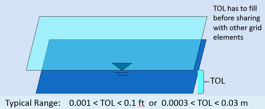
Figure 10. TOL Definition.

Grid Element Depression Storage that Must Be Filled Before Volume is Exchanged with Another Element

2.5.1. Previous Methods for Addressing Volume Evacuation

Any negative volume in floodplain or channel elements after the computational loop was previously redistributed to the other neighbor elements and the volume in the given cell was set to zero. This necessitated an extra computation loop for all the elements to re-sum all the volumes after the redistribution, but the timestep was not decremented. Instead, the normal computational routine continued uninterrupted but with an extra computational loop for all the grid elements for all timesteps. This was a computationally expensive approach. Addressing the volume evacuation issues required a review of the cells listed in the EVACUATEDFP.OUT and EVACUATEDCH.OUT files and adjusting cell attributes such as n-values, elevation, surface area or other features or components. Narrow inset low flow triangular channels were typically a problem and needed to be revised to a U-shaped channel that holds more volume at low flow depths. Correlating the grid elements listed in these files with those listed TIME.OUT enabled the most critical cells slowing down the model to be addressed first.

In addition, if the number of times evacuated elements on the floodplain reached 1,000, this caused the model to stop; presuming that this number of incidents of evacuated cells needed to be corrected. Often evacuated cells may be associated with discharge or water surface controls such as hydraulic structure or other components. The concept was to review the EVACUATEDxx.OUT files and adjust those evacuated element attributes before the final model product was completed.

2.5.2. Evacuated Element Revisions

Several codes revisions were made to simplify and automate the model response to evacuated elements including:

1. The separate computational loop for evaluating the evacuated cells was eliminated.

2. The limitation on the number of times (1,000) that evacuated elements were encountered was eliminated. The number of times each floodplain or channel element is now evacuated is listed in the EVACUATEDxx.OUT files.

3. Evacuated element n-values are increased by 0.001 to a limit of 0.250 for both the floodplain and channel.

4. The model terminates the current timestep loop and reduces the timestep by 1 percent.

5. The evacuated channel element TOL value is increased to 0.2 ft (0.067) if TOL is less than 0.2 ft (0.067 m) and increases the TOL by 0.02 ft (0.006 m) if greater than 0.2 up to a maximum value of 0.4 ft (0.122 m).

6. The floodplain evacuated element TOL value is increased to 0.1 ft (0.03) if TOL is less than 0.1 ft (0.03 m) and increases the TOL to 0.25 ft (0.076 m) if greater than 0.1 ft (0.03 m).

The focus is to adjust the flood hydraulics and the depression storage rather than the timestep for evacuated elements at shallow flows.

2.5.3. Reviewing the Evacuated Element Results

First review the SUMMARY.OUT and CHVOLUME.OUT file to see if there is any volume conservation error. Volume conservation error is not always related to evacuated elements, but it could be. Reviewing the EVACUATEDFP.OUT and EVACUATEDCH>OUT files and the TIME.OUT file will further help to identify if the model is not conserving volume in response to the evacuated elements. If EVACUATEDxx.OUT are empty or non-existent, the volume conservation error is being caused by some other component of the model. If the grid elements in these files are correlated, then review the ROUGH.OUT file to see if the same elements have increased n-values. When there are evacuated elements that are impacting the model performance, then it is necessary to review these elements in detail in terms of their attributes (n-values, elevations) or components (ARF-values, streets, infiltration, etc.) and make some adjustments. For these projects, only run the simulation until the model begins to slow down (a timestep less than 0.1 second or lower) and continue to adjust the evacuated elements until these no longer appear in the output files.

2.6. Limiting Froude Number

Using the Froude number in flood routing models is important to the both the understanding of the floodwave movement and the numerical stability of the model. It is even more important when considering mobile bed channels such as alluvial fans or high bedload rivers. The dimensionless Froude number Fr is given by:

(2.13)\[Fr = \frac{\text α^{0.5} V}{gd^{0.5}}\]

where:

V = depth averaged flow velocity

G = acceleration due to gravity

d = depth of flow above the thalweg

α = kinetic energy correction factor (involving the fluid density and specific weight). Typically α is assumed to be 1.

The Froude number helps to define the influence of gravity on the flow pattern. A low wave will propagate in free surface flow (open channel) depending only on the gravitational acceleration and the flow depth. The movement (speed) of the shallow wave, known as the wave celerity c = √gd, is related to average flow velocity through the Froude number. By accepting reasonable limitations of the overland (or channel) flow velocity and floodwave movement, the Froude number can be used to further define the relationship between the velocity and flow depth.

For essentially steady and uniform flow, the Manning’s n value is defined would be defined by:

(2.14)\[n = \frac{0.262}{F_r} d^{0.17} S^{o \, 0.5}\]

indicating that the flow roughness is inversely proportional to the Froude number. By assuming a reasonable limiting Froude number, the n value can be estimated from the normal depth and slope for a given flow discharge. In the FLO-2D model, the suggested n-value is based on either bankfull discharge for channel flow or 1 meter (3 ft) flow depth for overland flow (roughness is fully submerged). Suggested typical limiting Froude numbers are defined in Table 1.

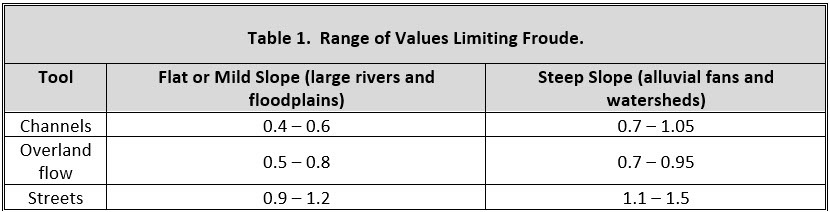
Table 1. Typical Limiting Froude Numbers.

Similar values are also reported in the CVFED FLO-2D Application Guide. If the limiting Froude number is exceeded, the grid element n-value increases by 0.001 for the next timestep. When limiting Fr is no longer exceeded, the n-value decreases by 0.0005 if it is greater than the original n-value. The changes in n-value reported in ROUGH.OUT, FPLAIN.RGH, CHAN.RGH and STREET.RGH files. The use of limiting Froude number in the FLO-2D model is documented in the FLO-2D Pocket Guide, the FLO-2D Reference Manual, and the CVFED FLO-2D Application Guide.

The maximum n-values for discretized models will be greater than typical n-values for HEC-RAS cross sections (both channel and overbank areas). This is because of the unsteady and non-uniform flow contribution between elements and the flow not being parallel to the cross section.

For flows over mobile bed conditions (supply unlimited), critical flows are approached asymptotically (Grant, 1997). A relatively steep slope is required for flow with sediment transport to achieve critical flow because the flow hydraulics oscillate. For Fr > 1, flow instability leads to rapid energy dissipation and bed erosion. Flow is forced to stay around critical by incipient motion thresholds. The equilibrium sand bed morphology tends to minimize the Froude number (Jia, 1990).

The limiting Froude number for mobile bed conditions can be approximated by (Grant, 1997):

(2.15)\[Fr = 3.85 \, S^{0.33} \quad \text{gravel bed} \quad \tau^{*}_{cr} = 0.03\]

(2.16)\[Fr = 5.18 \, S^{0.11} \quad \text{sand bed} \quad \tau^{*}_{cr} = 0.06\]

Roughness n-values include many factors: n = n1 + n2 + n3 + n4 + …such as friction drag, vegetation, expansion/contraction, bed forms, flow in bends, unsteady and non-uniform flow.