Hydrology

Learn how to set up rainfall and infiltration using QGIS and the FLO-2D Gila Plugin.

Note

It will be easier to view these videos on YouTube.

Set the video playback speed to 2x to complete the lessons faster.

The videos are more detailed whereas the text gives the minimum steps needed to complete the project.

Load the Project

This lesson shows how to load a FLO-2D project in QGIS, manage paths, and handle GeoPackage data.

Step 1: Launch QGIS

• Open the QGIS application.

Tip

To avoid searching for QGIS every time, right-click the QGIS icon and select “Pin to Start.”

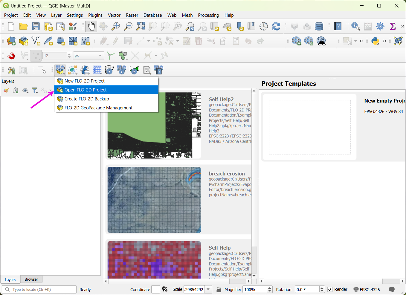
Step 2: Open Your Project

• If QGIS opens the most recent project, simply click on it in the Recent Projects list.

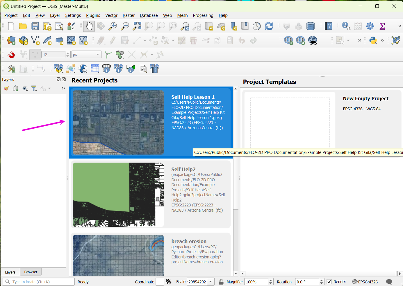
• If the project was moved and no longer loads:

  • Go to Plugins > FLO-2D > Open FLO-2D Project.

  • Navigate to the project .gpkg file (GeoPackage) and select it.

Note

The GeoPackage contains the entire project, including the .qgz file.

Assign an Inflow Node

This tutorial shows how to create an inflow boundary condition at a project edge where an upstream channel—Cave Creek—enters the basin. This is useful when modeling runoff entering the system from offsite.

Step 1: Navigate the Map

• Use the mouse scroll wheel to zoom in and out.

• Click and drag with the middle mouse button (wheel) to pan the map view.

Step 2: Add an Inflow Node

• In FLO-2D Panel, click Collapse All to clear any open panels.

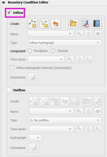
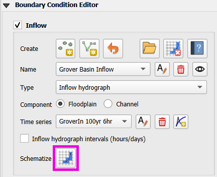
• Expand Boundary Condition Editor.

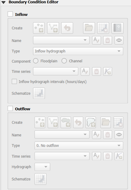
• Choose the Inflow Node option.

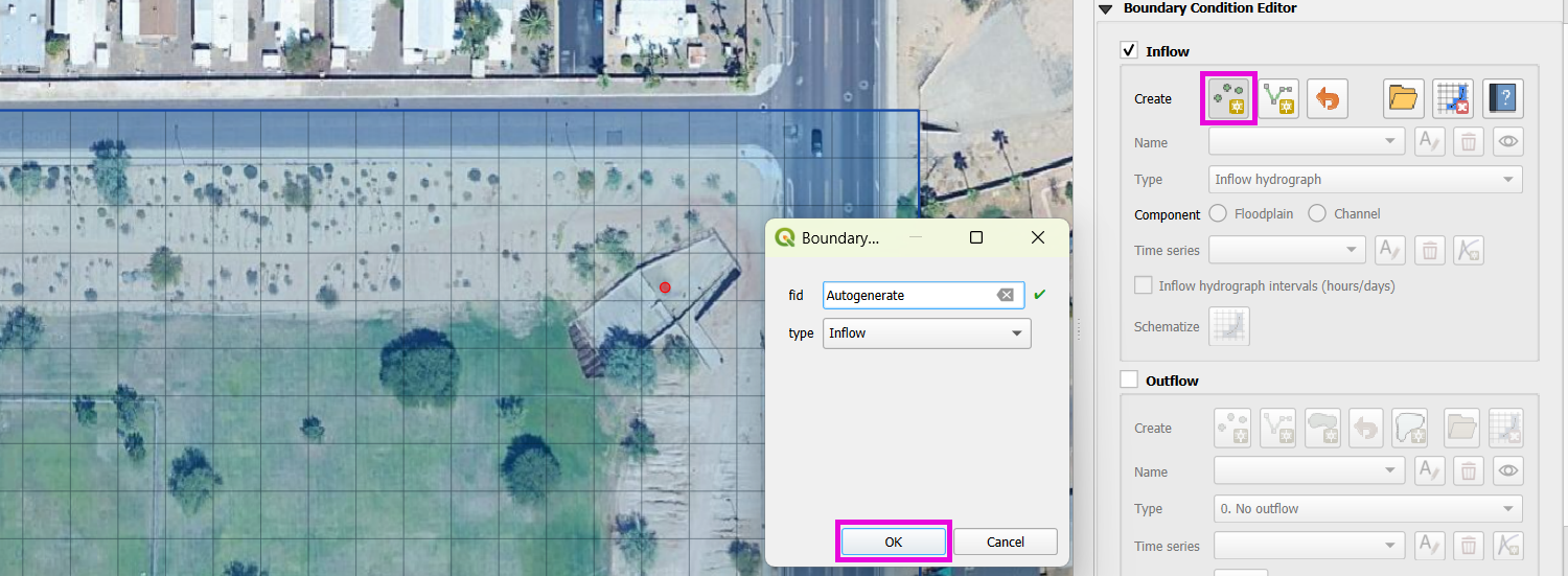
• Click Add Point, then click on the map at the outlet of the structure (culvert with dissipator and grate).

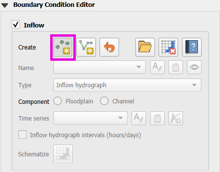
• Click OK to create the inflow point, and then click the Add Point button again to save it.

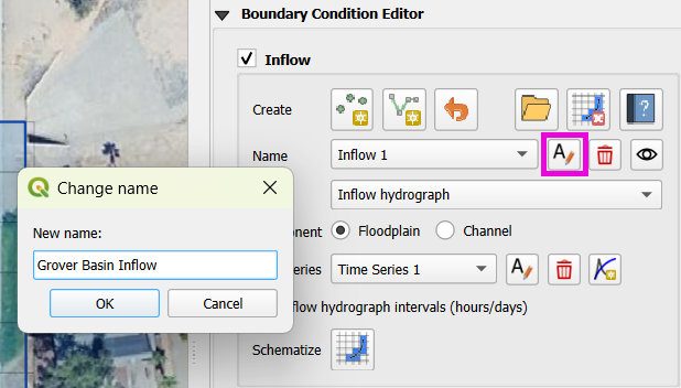
Step 3: Rename the Inflow Point

• Click Rename, and rename to “Grover Basin Inflow”

Step 4: Create a Time Series

• Go to the Time Series Editor.

• Click Rename, and rename “Time Series 1” to “GroverIn 100yr 6hr”

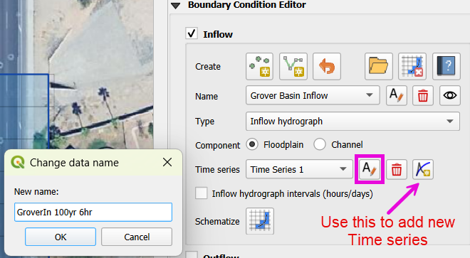
• This is a 100-year, 6-hour inflow hydrograph taken from the original larger project.

• Set the Type to: Floodplain

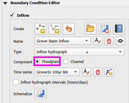
Warning

Do not select Channel unless modeling a 1-D FLO-2D channel. This is surface runoff entering the basin.

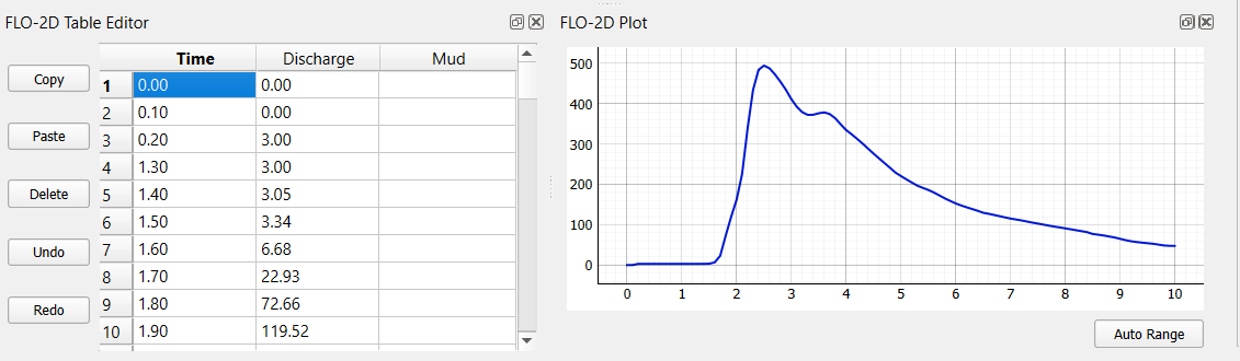
Step 5: Paste Hydrograph Data

• Open the provided hydrograph data file from Lesson 1 Data.

• Choose the 100yr 6hr inflow file.

  

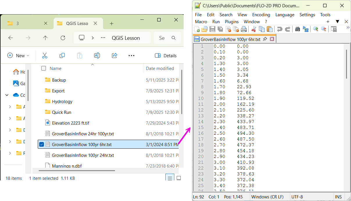
• Time should be in hours on the left and discharge (cfs) on the right.

• Select all data with Ctrl+A, then copy with Ctrl+C.

• Close the file with Ctrl+W.

• In the QGIS Time Series Editor, click the first cell and paste using Ctrl+V.

Note

FLO-2D uses cubic feet per second for discharge unless the metric units switch is on, in which case it uses cubic meters per second.

Step 6: Schematize the Data

• Click Schematize to convert the pasted user input into FLO-2D schema data.

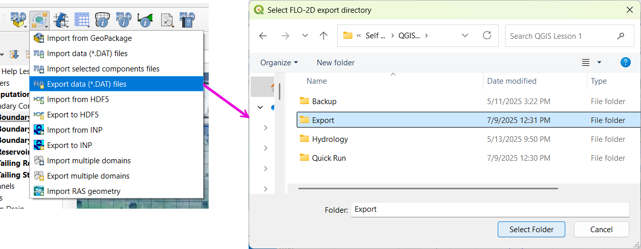
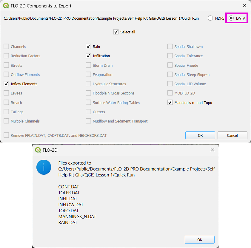
Step 7: Export the Inflow File

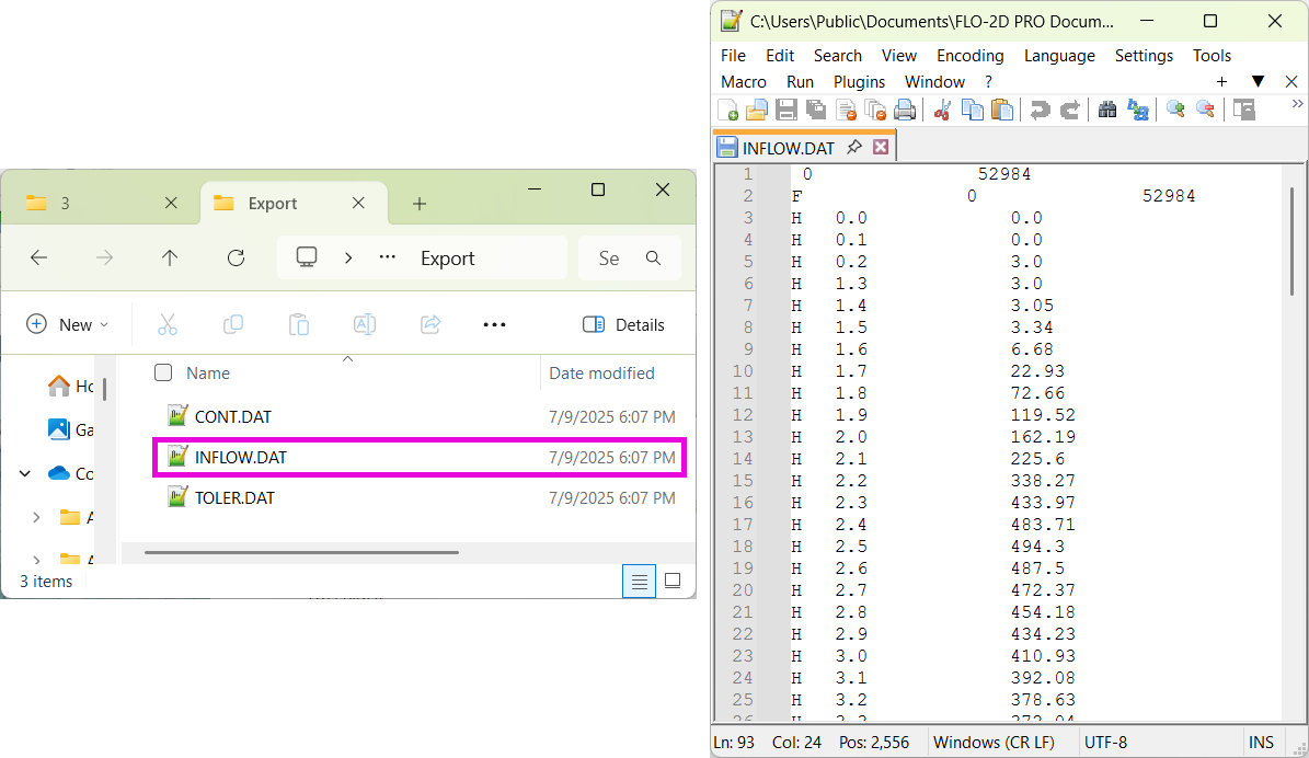
• Right-click the inflow node and choose Export > Data.

• Set the export folder and confirm.

• Select only the Inflow Elements, not all files.

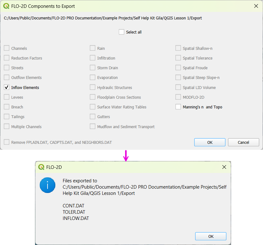
You will now have a file called INFLOW.DAT.

Assign Rainfall

Step 1: Open the Rain Editor

• In FLO-2D Panel, click Collapse All to clear any open panels.

• Expand Rain Editor.

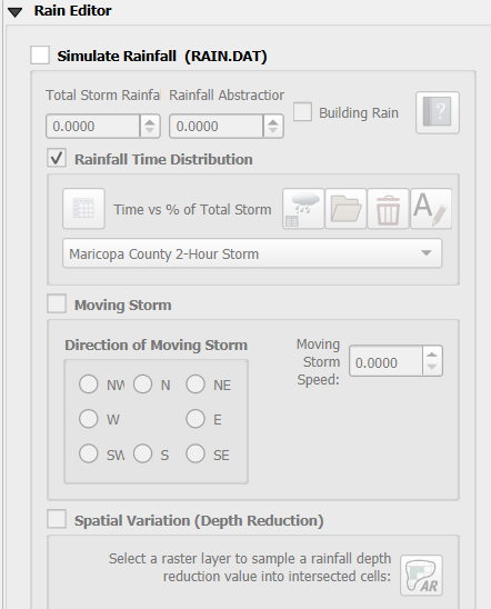
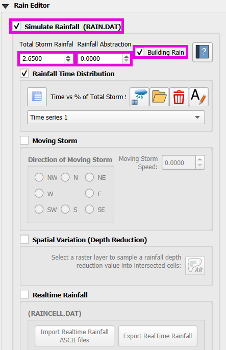
• Check Simulate Rainfall.

• Set the Total Rainfall Depth to 2.65 in (this example uses a 6-hour, 100-year event).

• Leave Rainfall Abstraction at 0.0 for now. This is set elsewhere.

• Check Apply Building Rain.

Step 2: Add a Storm Pattern

• Click Open next to the storm pattern.

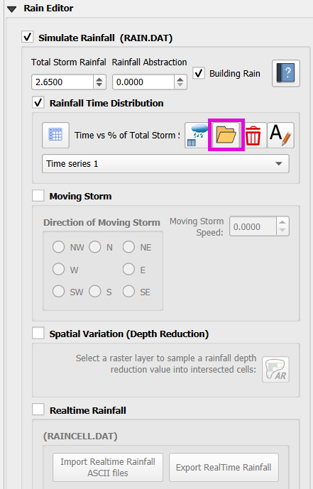
• Navigate to the FLO-2D documentation folder and find the 6-hour event distribution. Choose the first pattern from the list.

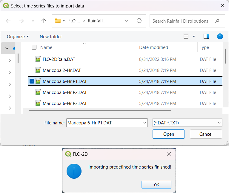
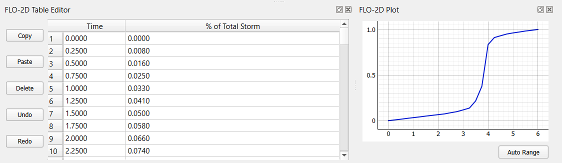
• Confirm the time-percent curve was imported correctly.

Important

The rainfall distribution table has:

• Time (hours) on the left.

• Cumulative rainfall (0–1) on the right.

The percent values must start at time = 0 and rainfall = 0.

Step 3: Understanding Rain on Grid

• Rainfall is applied uniformly across all grid elements.

• Every element receives 2.65 inches following the selected pattern.

• This is called “rain on grid”, and it is different from assigning rainfall to subcatchments.

Tip

Rain on grid works well for small projects. For large areas, continue to Step 4.

Step 4: Sample a Rainfall Raster (Optional)

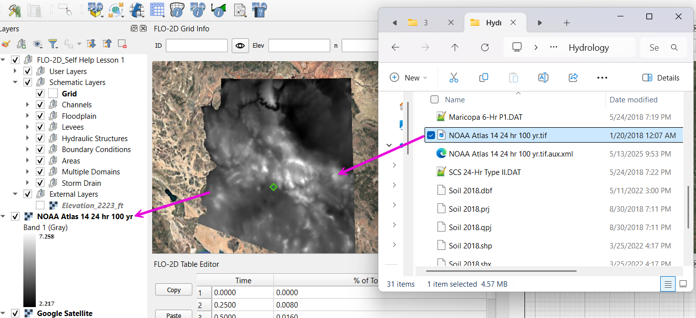
• NOAA Atlas 14 rainfall raster cab be used to apply spatially variable rainfall as described in the following steps.

  • Drag the 24-hour rainfall raster into QGIS.

  • Right-click the layer > Zoom to Layer.

  • Check the data: it should be in inches and match the coordinate system in use.

  

• To apply the raster:

  • Go to the Rain Editor.

  • Check Sample from Raster.

  

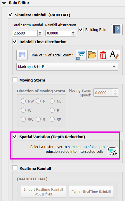
  • Select NOAA Atlas 14 rainfall raster file.

  • Leave “Fill NoData” unchecked if not needed.

  • Click OK and confirm.

  

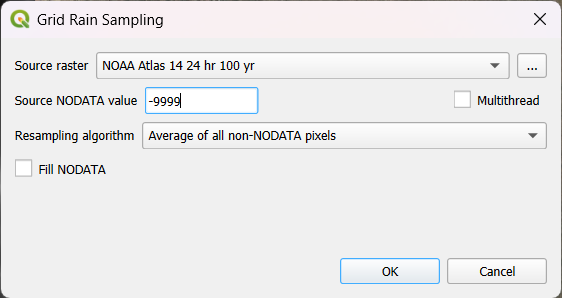
• QGIS will now sample rainfall values from the raster to each grid element based on spatial location.

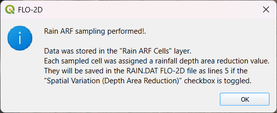
Note

The sampling uses the centroid of each grid element and computes a point reduction factor based on the maximum raster value. It is not a depth-area reduction, but rather a point-based rainfall adjustment.

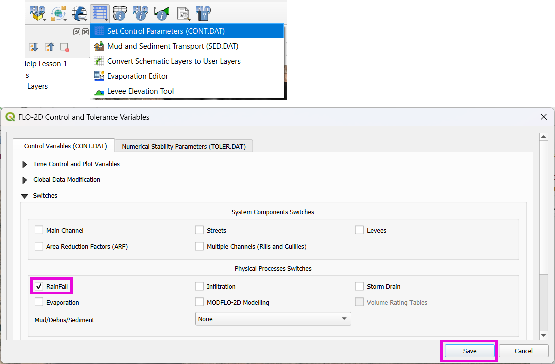
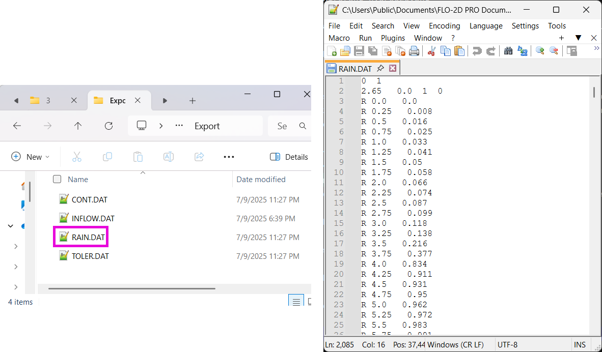
Step 5: Export Rainfall Data

Check Control Parameters:

• The rainfall switch is turned on automatically when Simulate Rainfall is checked. Click Save.

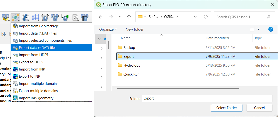
• Export DAT Files.

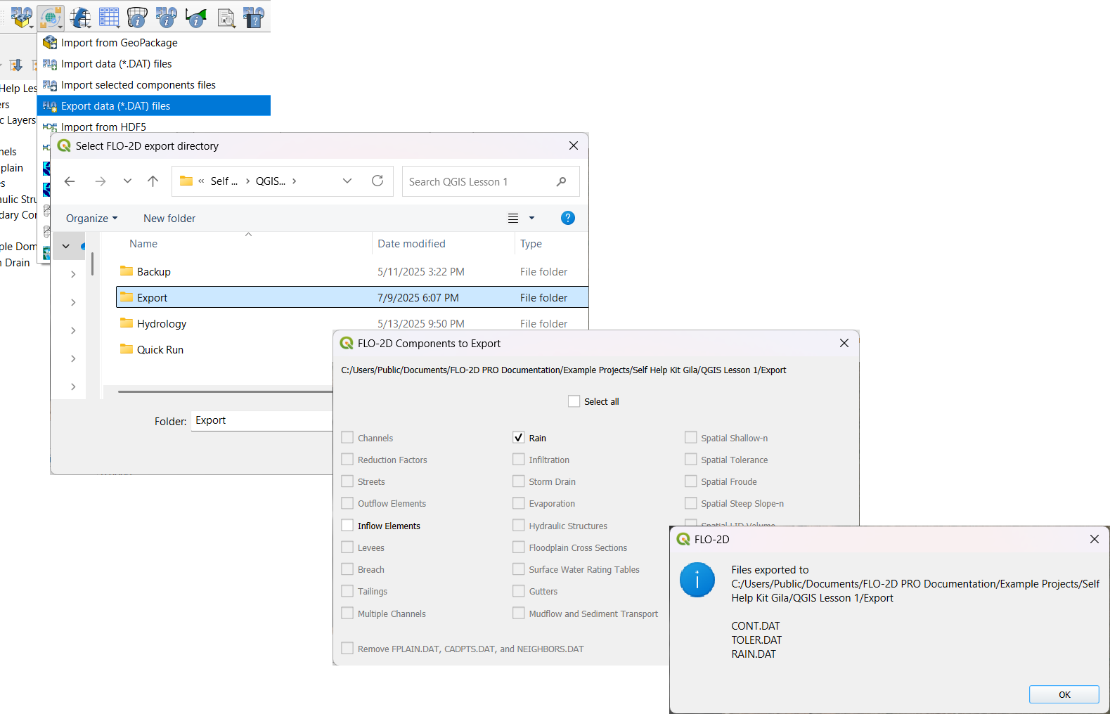
• This will generate a RAIN.DAT file in the export folder.

Infiltration

Important

FLO-2D uses three infiltration types. Choose one lesson and skip the other two.

Infiltration - Assign Green and Ampt

This lesson walks through the Green-Ampt infiltration method in FLO-2D, including the 2018 and 2023 Flood Control District methods and the SSURGO/OSM-based method. It covers how to set global parameters, apply land use and soil data, and export Green-Ampt data files.

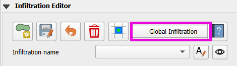
Step 1: Set Global Parameters

• Open the Global Infiltration tool.

• Check Green-Ampt.

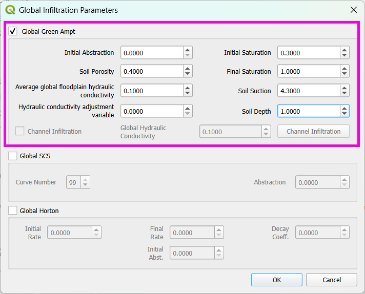
• Click OK.

Step 2: Load Land Use and Soil Shapefiles

• Add land use and soil shapefiles (e.g., 2018 or 2023 Maricopa County).

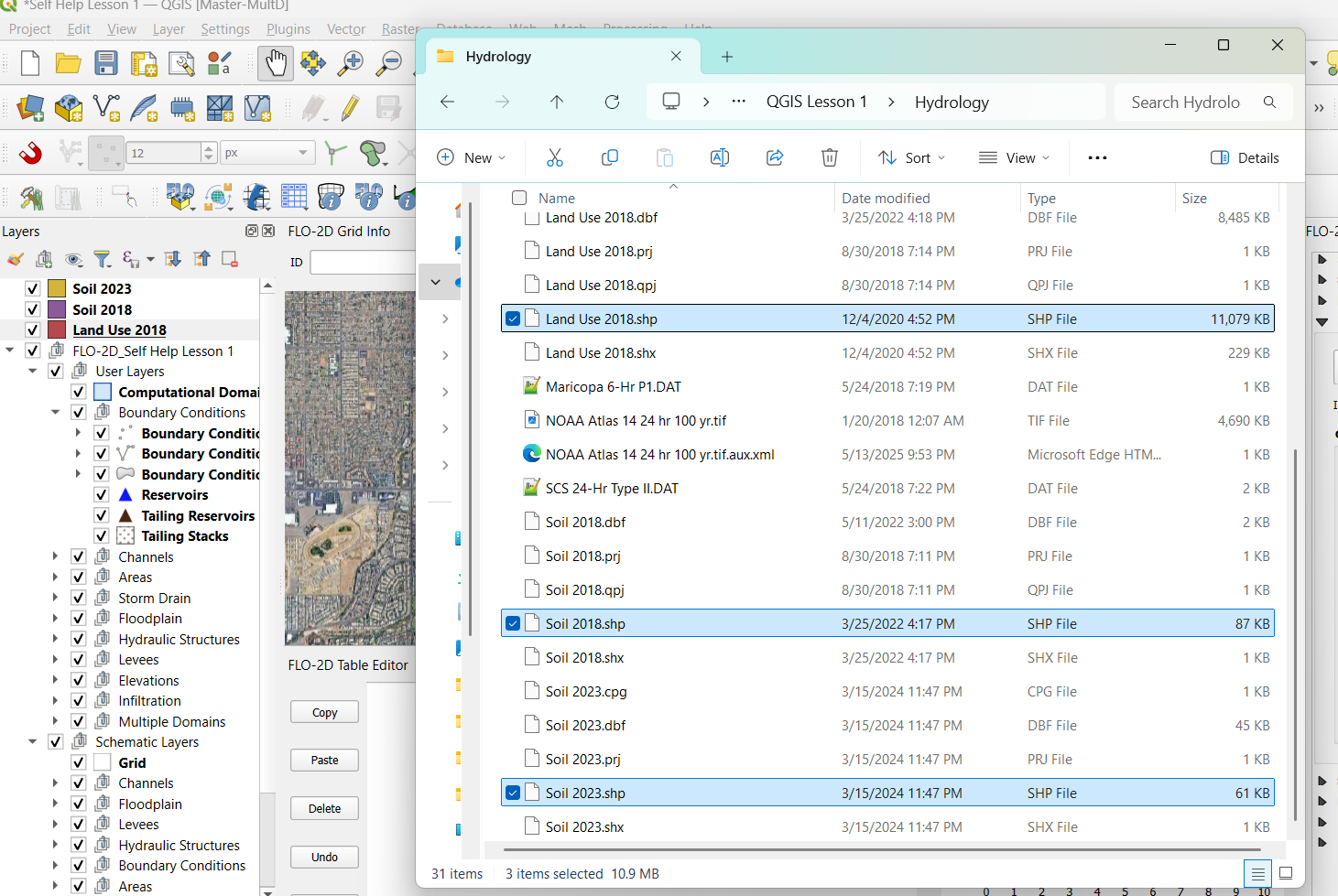
• Inspect attributes such as: - initial abstraction, impervious, initial saturation - hydraulic conductivity (XKsat), soil depth - DTheta dry, DTheta normal, Psif

Step 3 (Option 1): Use the 2018 Method

• Run Green-Ampt Calculator (2018 version).

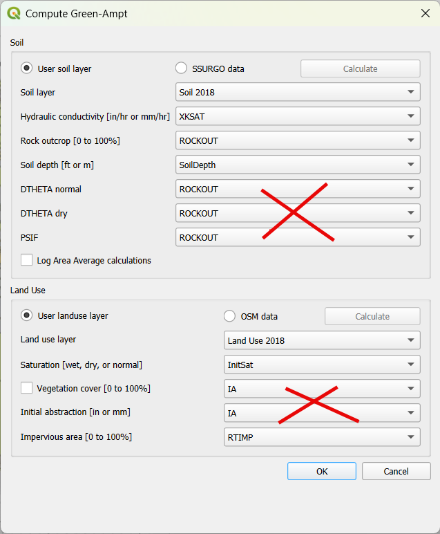
• Input Fields:

  • Soil Layer: XKsat, RockOutcrop, SoilDepth

  • Land Use: Initial Saturation, Initial Abstraction, Impervious

  • Leave Vegetative Cover unchecked.

• Click OK to calculate.

• Review the 2018 Manual Settings:

  • 2018 method derives Psif and DTheta from XKsat.

  • Uses area-weighted averages (no log scaling).

  • Global and local infiltration data will be stored in INFIL.DAT.

• Step 5: Export Infiltration Data

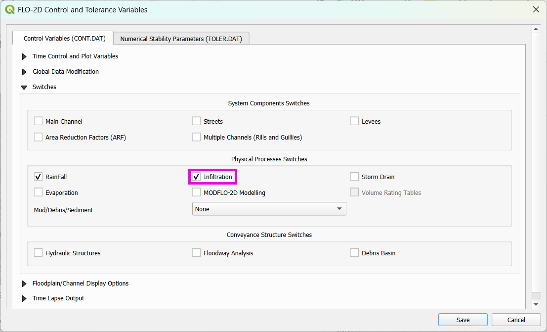
  • Ensure Infiltration Switch is ON in Control Parameters.

  

  • Click Export DAT Files.

  

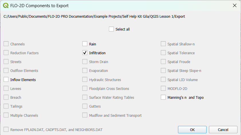
  • Export only INFILTRATION and CONT.DAT.

  

Step 3 (Option 2): Use the 2023 Method

• Switch calculator to use 2023 soil shapefile.

• Input Fields:

  • Soil Layer: XKsat, RockOutcrop, SoilDepth, DTheta Normal, DTheta Dry, Psif

  • Land Use: Initial Saturation, Initial Abstraction, Impervious

• Leave Vegetative Cover unchecked.

• 2023 method uses:

• Log area average for XKsat and Psif

• Intersected DTheta from land use-soil overlay

• Maximum impervious value from both layers

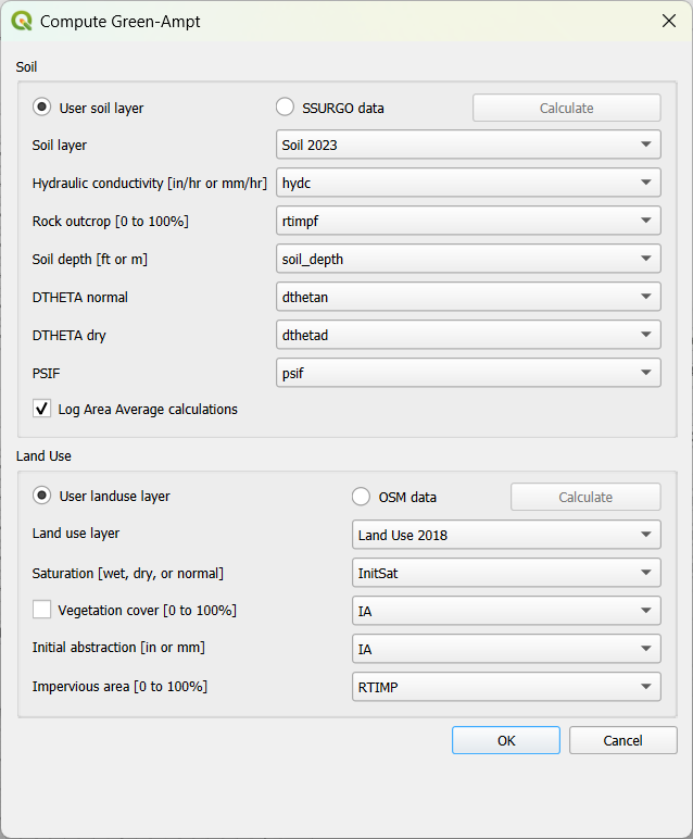
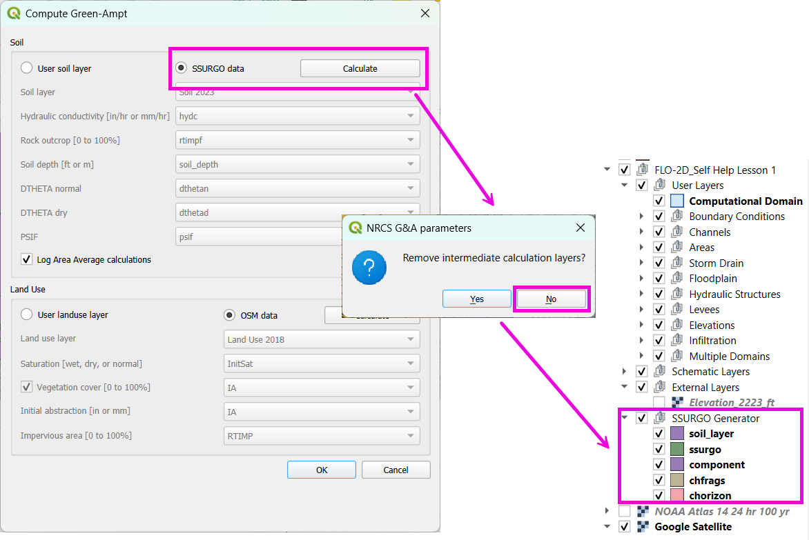
Step 3 (Option 3): Use SSURGO and OpenStreetMap Data

• Use SSURGO Downloader to get soil components:

  • Horizon, Fragmentation, Component layers

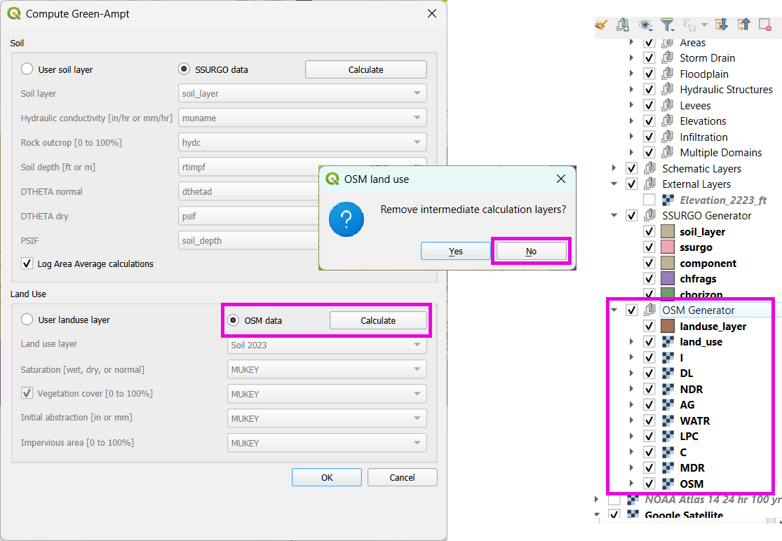
• Use OSM Downloader to generate land use polygons:

  • Raster images are vectorized based on color mapping.

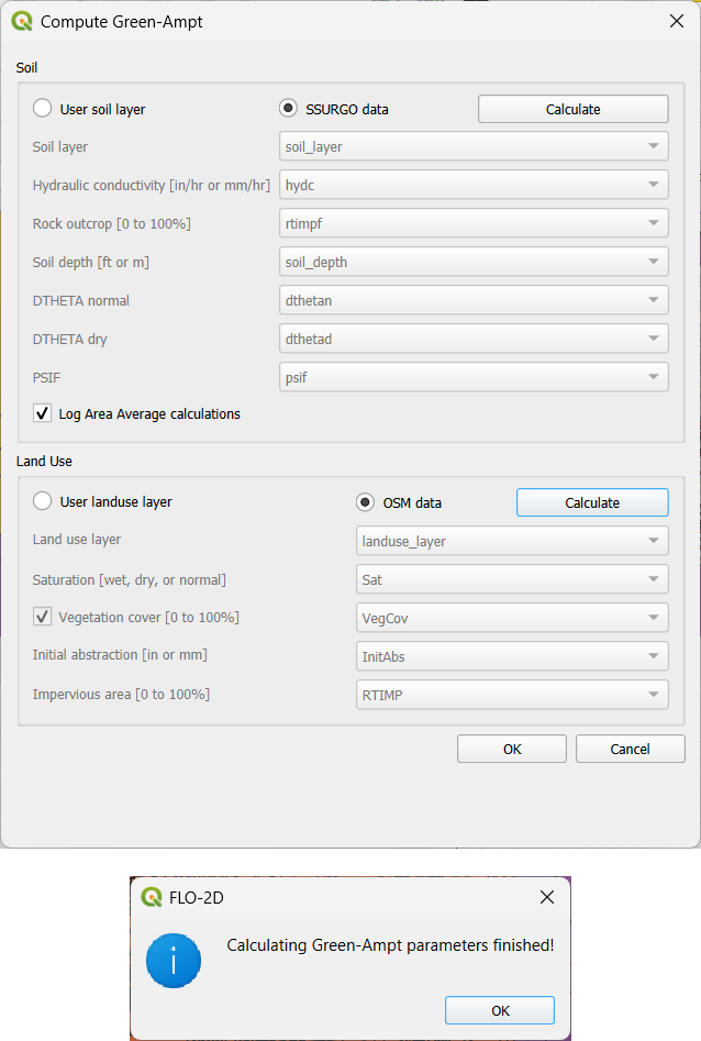
• Calculator reads attributes:

  • Land Use: Initial Saturation, Impervious, Initial Abstraction

  • Soil: XKsat, Soil Depth, DTheta, Psif

Step 8: Verify Infiltration Attributes

• Enable Advanced Layers in FLO-2D Settings.

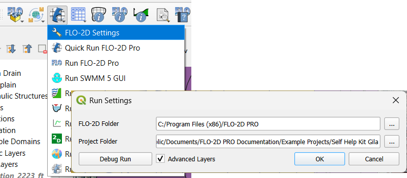
• Review attributes in infiltration_results:

  • Hydraulic Conductivity

  • Soil Suction

  • DTheta

  • Initial Abstraction

  • Impervious

  • Soil Depth

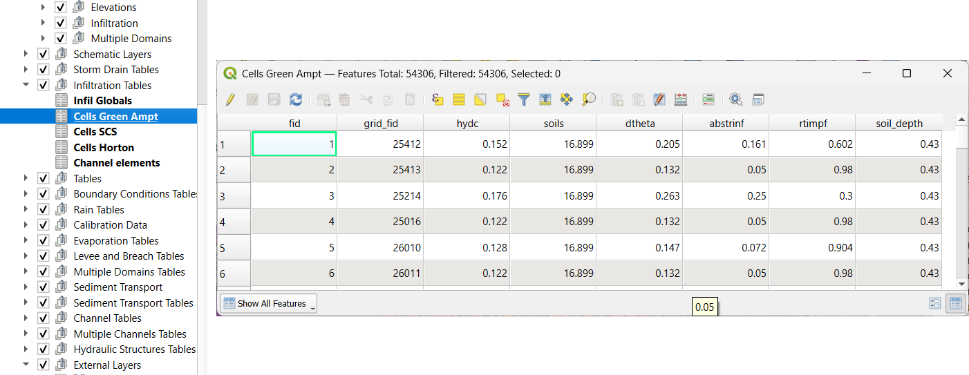
Note

Always re-sort by FID before export to avoid misaligned data rows.

Infiltration - Assign SCS Curve Number

Step 1: Generate Curve Number Layer

• Open the Curve Number Generator from the Toolbox.

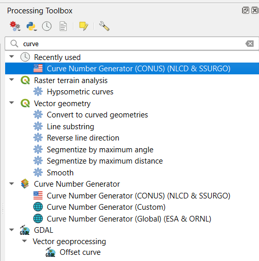
• This downloads and intersects:

  • NLCD land cover data

  • SSURGO soil data

• Set outputs to Temporary Layers, except save the final Curve Number layer.

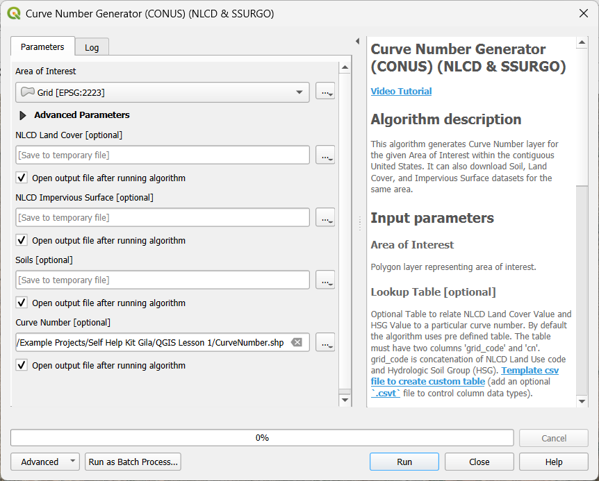
• Click Run to create your composite Curve Number layer.

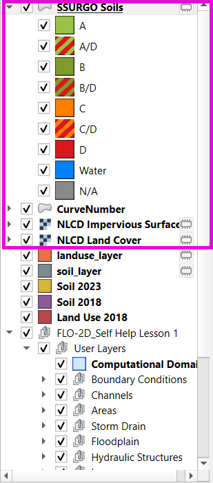
Step 2: Inspect Generated Layers

• You’ll see several layers:

  • Soils layer (SSURGO)

  • Impervious surface raster from NLCD

  • Land cover classification

  • Final Curve Number layer

Tip

Use the Identify Features tool to inspect pixel values, such as percent impervious or land class (e.g., “Developed, Open Space”).

Step 3: Edit Curve Number Values

• Open the Attribute Table of the Curve Number layer.

• Use field calculator or manual selection to edit curve numbers.

• Example: Select polygons with Curve Number < 63 and update to 63.

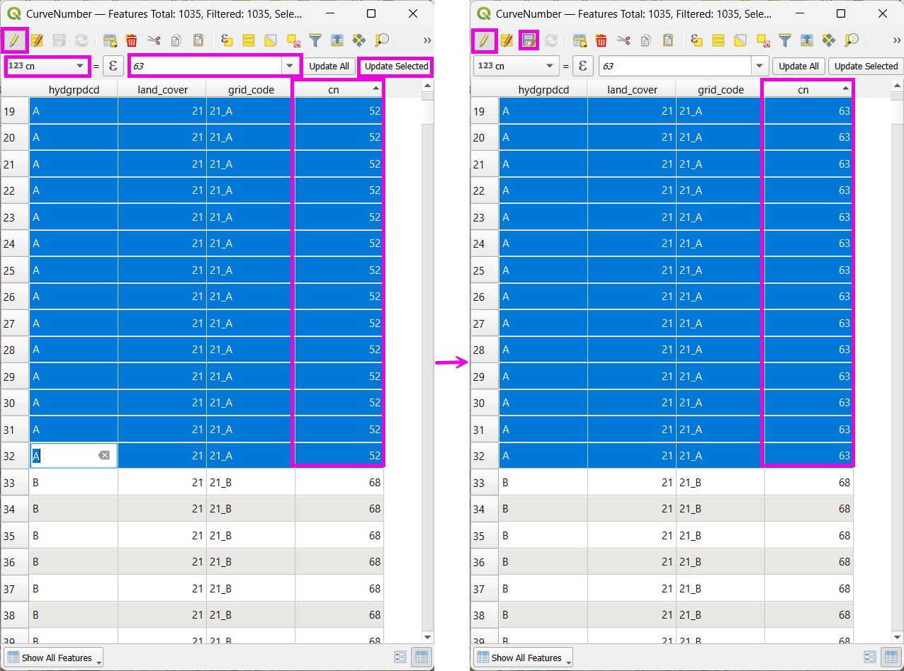
• Save edits and close the attribute table.

Step 4: Apply Curve Number to Grid

• Open Infiltration Editor > Global Infiltration.

• Choose Curve Number as your method.

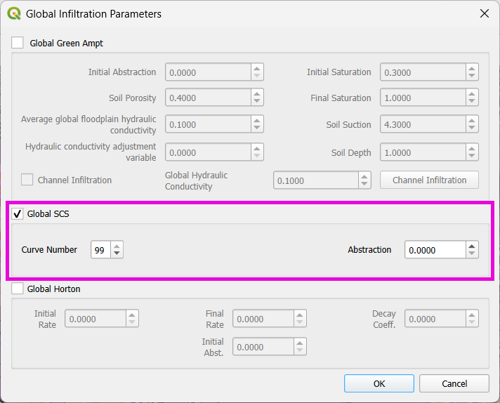
• Click OK.

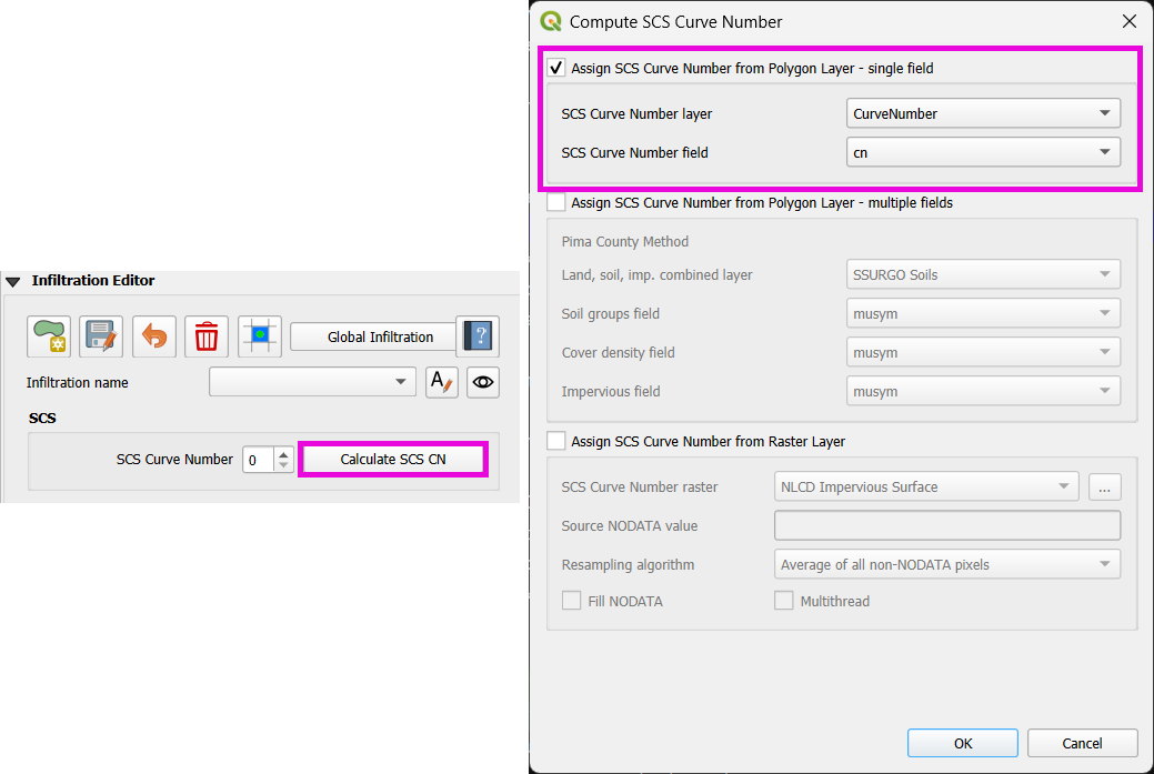
• Now go to Calculate Curve Number:

  • Select the Curve Number layer

  • Choose the correct field

  • Apply values to the grid.

Step 5: Export Infiltration Data

• Enable the Infiltration Switch in Control Parameters.

• Save your control settings.

• Go to Export DAT Files.

• Select only Infiltration and export.

Note

INFIL.DAT will include: - Switch = 2 for Curve Number method - Global values (optional) - Local values per grid element

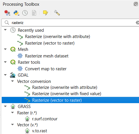
Step 6: Optional - Rasterize Curve Number

If the Curve Number polygon layer is too complex or fragmented:

• Open Rasterize Vector to Raster from the Processing Toolbox.

• Input:

  • Layer: Curve Number shapefile

  • Field: Curve Number

  • Cell size: 30 x 30

  • Extent: Match your FLO-2D grid layer

  • No Data value: -9999

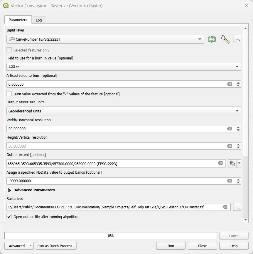
• Save output raster and click Run.

Step 7: Use Raster Calculator (Alternative Method)

• Open Infiltration Editor > Curve Number from Raster.

• Select your rasterized Curve Number layer.

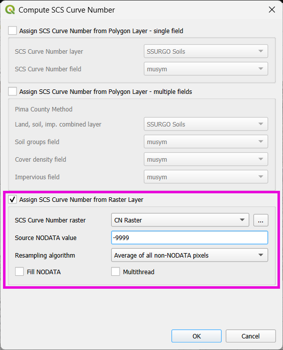
• Click OK to apply sampled values.

Note

Raster sampling uses the centroid of each grid element to pull the value and applies a point-based reduction.

Infiltration - Assign Horton

Step 1: Prepare Horton Shapefile

• If you don’t have Horton data, you can estimate it by comparing with SCS Curve Number values.

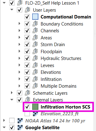
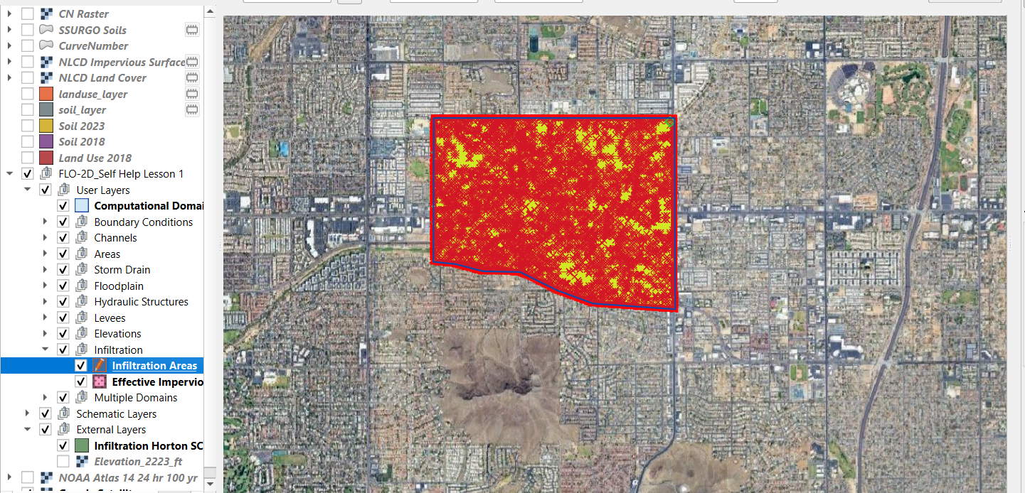
• Create a shapefile with estimated Horton parameters.

• Add this shapefile to QGIS and place it in the External Layers group.

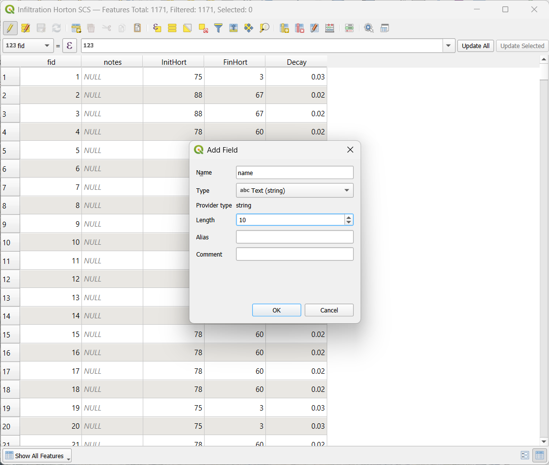
Step 2: Add Unique Name Field

• Open the Attribute Table and toggle editing.

• Add a new field named name (type: String).

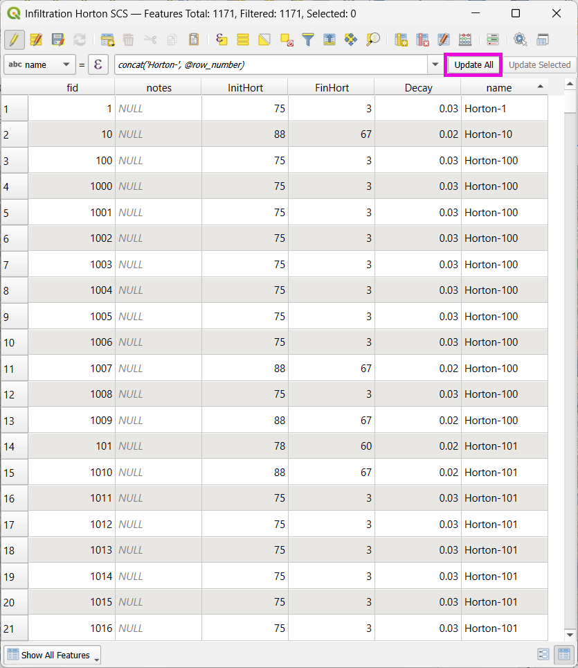
• Use the Expression Editor to generate unique IDs:

  • Use concat(‘Horton-’, @row_number) to fill the field.

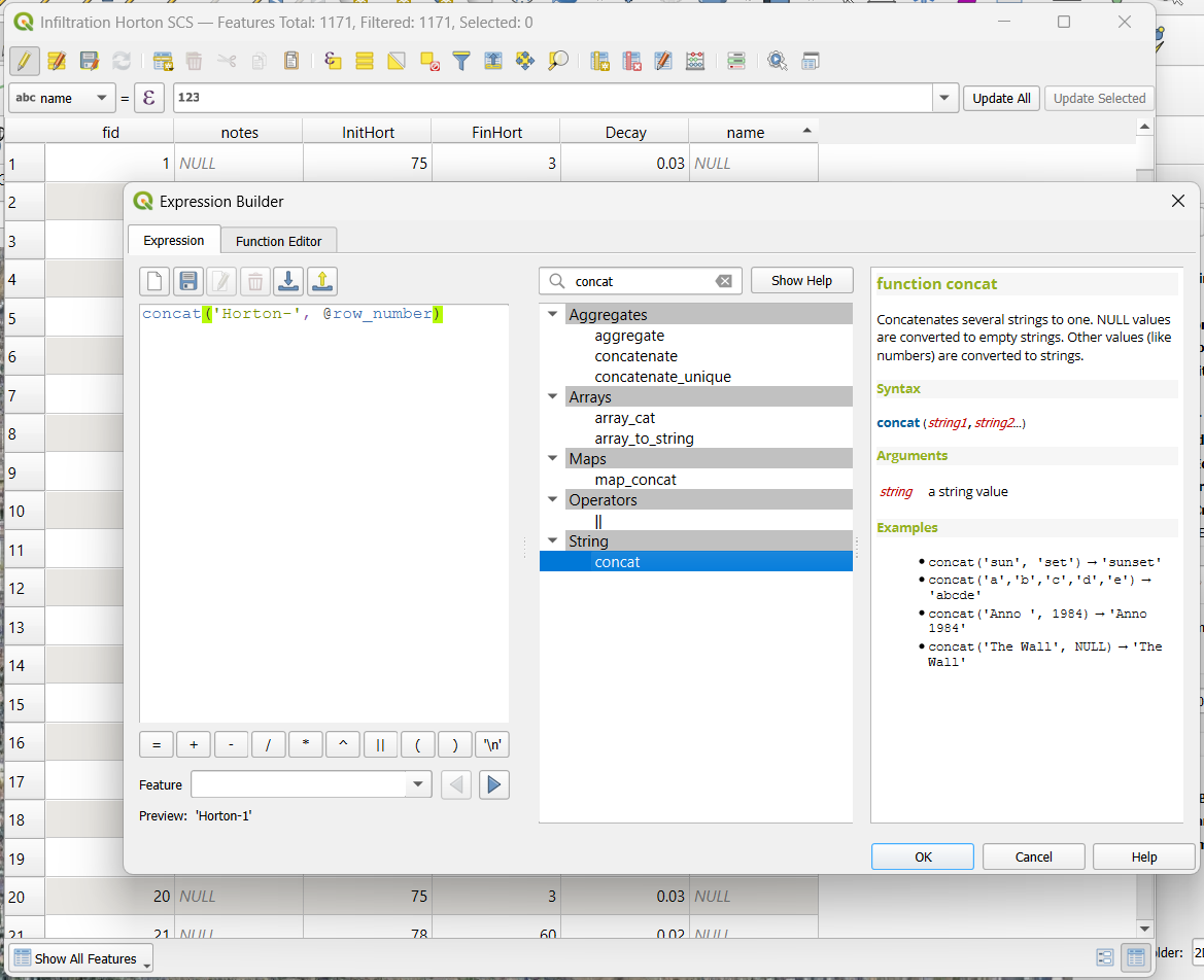
• Click Update All, save edits, and stop editing.

Step 3: Copy Features to GeoPackage

• Select all features in the shapefile.

• Press Ctrl+C to copy.

• Edit the infiltration areas layer in your GeoPackage.

• Paste the features and save.

Note

Attributes are not copied. You will perform a table join next.

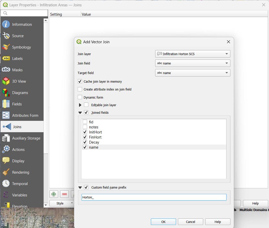
Step 4: Perform Table Join

• Right-click infiltration areas > Properties > Joins.

• Add a join to the Horton shapefile using the name field.

• Select only required fields: initial, final, decay.

• Add a prefix like Horton_ for clarity.

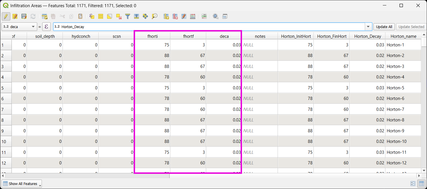
Step 5: Copy Joined Data

• Reopen the attribute table for infiltration areas.

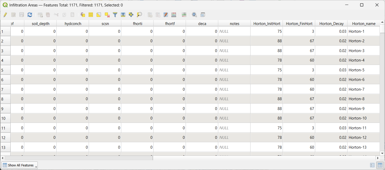
• Toggle editing and update:

  • Set Horton Initial = Horton_initial

  • Set Horton Final = Horton_final

  • Set Decay = Horton_decay

• Click Update All, save edits, and turn off editing.

Important

Joined fields are read-only. You must copy them to editable fields.

Step 6: Delete the Join

• Go back to Layer Properties > Joins.

• Remove the join to improve performance.

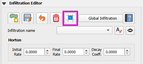
Step 7: Global Horton Parameters

• Open Infiltration Editor > Global Infiltration.

• Check Horton and enter generic global values (used only for missing cells).

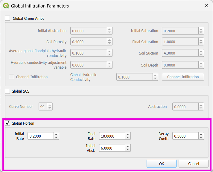
• Click OK.

Step 8: Schematize and Export

• Click Schematize to sample Horton values to the grid.

• Enable Infiltration Switch in Control Parameters.

• Save your project.

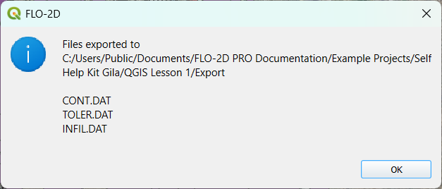
• Go to Export DAT Files.

• Select only INFILTRATION and CONT.DAT.

• Click OK to export.

Save Export and Run

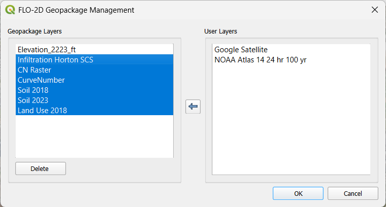
Step 1: Save Your Project

• Right-click any temporary layers are no longer necessary and select Remove.

• Click the Save Project button.

• When prompted, click Yes to save scratch layers into the GeoPackage.

This ensures they are committed and safely stored with the project file.

Step 2: Export Data Using Quick Run

• Use Quick Run to export and simulate in one step.

• Quick Run is only available if the project does not include storm drains.

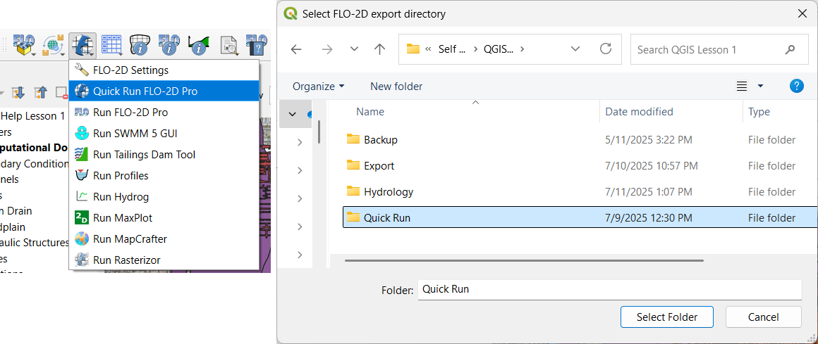
• To use Quick Run:

  • Click Quick Run from the FLO-2D toolbar.

  • Create a new folder (e.g., quick_run) for the export.

  • Select this folder when prompted.

Note

The Build 26 FLO-2D engine is capable of running models with *.DAT or input.hdf5 formats.

• The plugin will:

  • Export all required .DAT files

  • Automatically launch the simulation upon successful export

Step 3: Wait for Simulation to Start

Once data is exported, the model will begin running.

• Watch for early rainfall values in the results window.

  • Rainfall accumulation (e.g., ~0.1 in) will appear first.

  • Ponded water will start appearing on the grid.

  • Water will flow down streets and terrain according to the grid and infiltration settings.

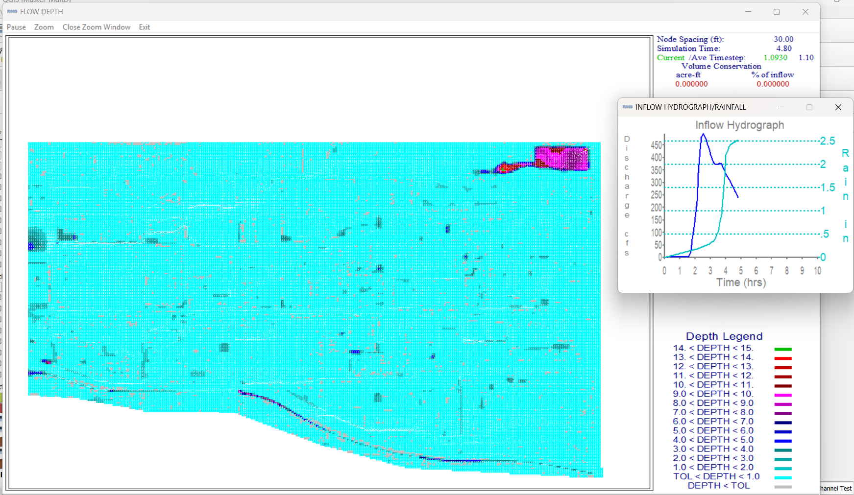
Note

Simulation results should show flow routing from rainfall across your modeled surface and toward low-lying areas.