
SCS#
FLO-2D uses three infiltration method. Green_Ampt, SCS, and Horton infiltration data development is outlined in this section. The INFIL.DAT file contains the infiltration data. The data can be global (uniform) or spatially variable at the grid element resolution. Global data is applied uniformly to all grid elements and spatially variable data allows different parameters to be applied to individual cells or groups of cells. The different methods for setting up the data are defined below.
Global Uniform Infiltration#
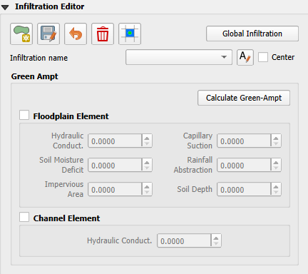
The SCS infiltration editor can add global or spatially variable infiltration data to the INFIL.DAT file for infiltration curve numbers.
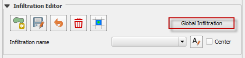
Set up the Global Infiltration first. Click Global Infiltration.
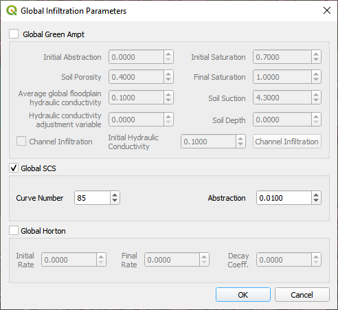
Fill the Global Infiltration dialog box.
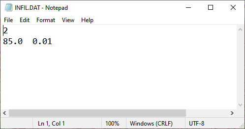
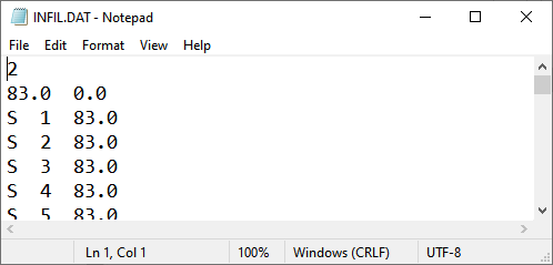
The INFIL.DAT file looks like this:
Where the infiltration type is 2 = SCS infiltration.
The 85 is the uniform curve number for each grid.
The 0.01 is the initial abstraction.
Spatial SCS Infiltration from Infiltration Areas User Layer#
Note
This method is the most effective way to sample SCS data. If using the other calculators, review SCS column for errors.
Spatially variable floodplain infiltration is set by digitizing infiltration polygons or importing infiltration polygons. Use the polygon editor to digitize spatially variable infiltration. Create a polygon to represent an area of infiltration.
Select the Infiltration Areas user layer.
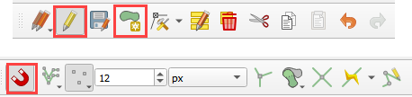
Click the editor pencil and snapping magnet button.
Create the polygons the represent areas with the same curve number.
Fill the table for the infiltration data.
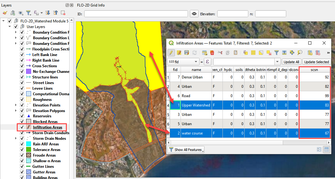
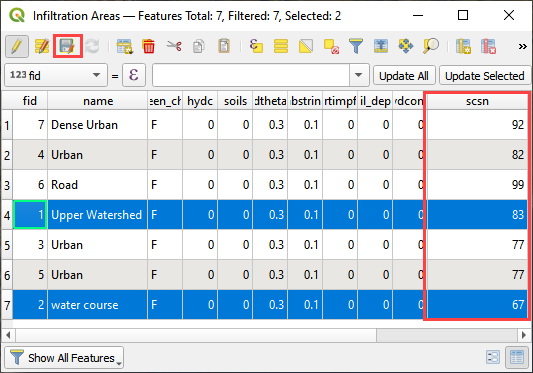
The finished table has a CN for every polygon.
Click the Save button to save the attributes.
Click the pencil button to close the editor.
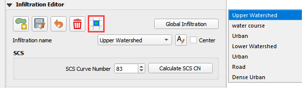
Check the data in the Infiltration Editor Widget. Click the Schematize button to complete the process.
The spatially variable INFIL.DAT looks like this:
Curve Number Generator#
If necessary, add the Plugin Curve Number Generator.
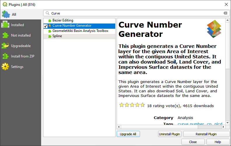
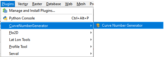
Open the Curve Number Generator.
Set the Area Boundary to the Grid. Check the boxes and click OK.
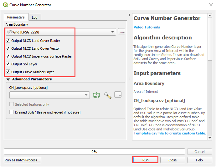
Click Close when process is finished. The Curve Number Polygon Layer can be used in the next section.
SCS Calculator From Single Shapefile#
Warning
If applying this method, review min and max of the SCS field. This method only works on polygon shapefiles that have no geometric deficiencies. If this method results in errors, copy the polygons to the User layer field and use the User Layer Method.
This option will add spatially variable infiltration data to the grid from a shapefile with one CN attribute field.
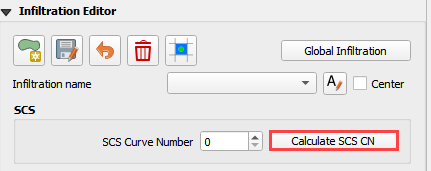
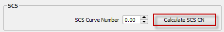
Click the Calculate SCS CN button.
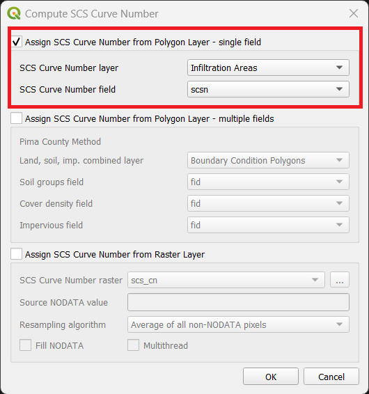
Check the ‘Assign SCS Curve Number from Polygon Layer - single field’.
Select the layer and field with the infiltration data.
This method works for shapefiles that have a CN already calculated.
Click OK to calculate a spatially variable CN value for every grid element.
When the calculation is complete, the following box will appear. Click OK to close the box.
The INFIL.DAT file looks like this.

SCS Calculator From Single Shapefile Multiple Fields Pima County Method#
Use this option for Pima County to calculate SCS curve number data from a single layer with multiple fields. This is a vector layer with polygon features and field to define the landuse/soil group, vegetation coverage and impervious space. This option was developed specifically for Pima County.
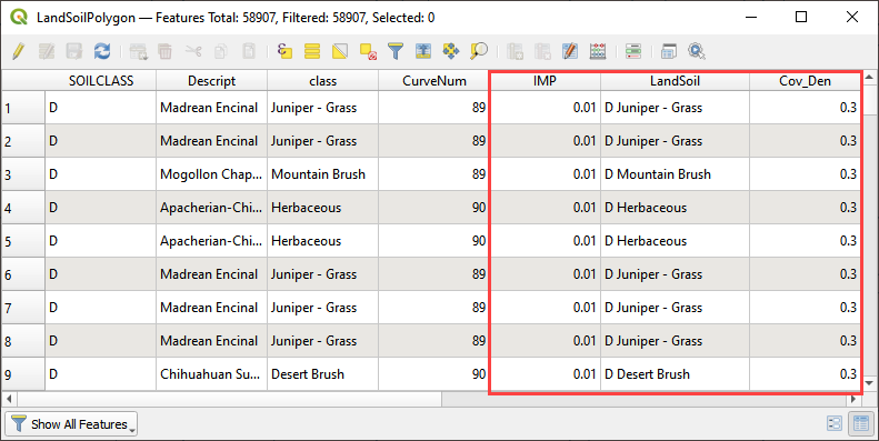
The data should be arranged as shown in the attribute table.
Click the Calculate SCS CN button.
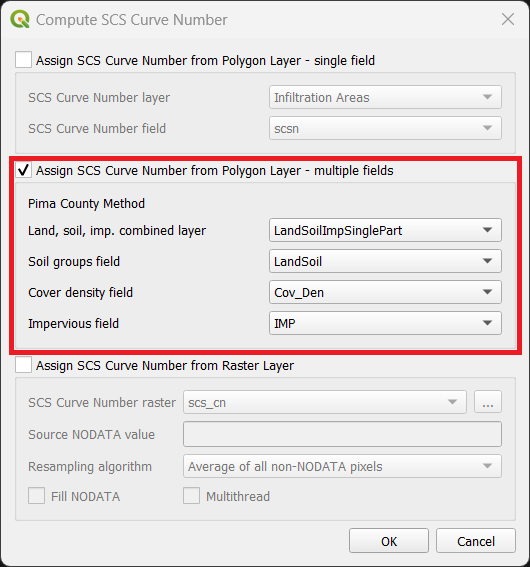
Check the ‘Assign SCS Curve Number from Polygon Layer - multiple fields’.
Select the layer and fields with the infiltration data and click OK to run the calculator.
When the calculation is complete, the following box will appear. Click OK to close the box.
The INFIL.DAT file looks like this.
SCS Calculator From Raster Layer#
This option will add spatially variable infiltration data to the grid from a raster with cells containing CN values. Important properties:
Important
The raster must have the same coordinate reference system (CRS) as the project. If the CRS is missing or is set by the user, save the raster with the correct CRS.
The best resolution of the grid element CN is achieved when the CN raster pixel size is smaller than the grid element size.
The raster warp method uses a weighted average to warp the original raster pixels to the cell size pixels.
Click the Calculate SCS CN button.
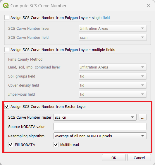
Check the ‘Assign SCS Curve Number from Raster Layer’.
Select the raster containing CN values from the dropdown or choose a raster from the file dialog.
Set the NODATA value.
Select the resampling algorithm.
Select the Fill NODATA option to set the CN of empty grid elements from neighbors. This is only necessary if there are empty raster pixels.
Select the multithread option to use all CPU’s for running the algorithm.
Click OK to calculate a spatially variable CN value for every grid element.
When the calculation is complete, the following box will appear. Click OK to close the box.
The INFIL.DAT file looks like this.
Troubleshooting#
Infiltration calculators all use intersection tools. This can cause problems if the shapefiles are not set up correctly. Specifically, land use and soils shapefiles that may have been converted from raster data. If errors persist, try “fix geometry”, “simplify”, and “dissolve” on the source shapefiles. These tools are part of the QGIS Processing Toolbox. They can also be corrected in ArcGIS if the datasets are very large.
Make sure the shapefiles completely cover the grid. If a grid element is outside the coverage of the infiltration, QGIS will show an error.
Make sure the shapefile fields have a correctly defined number type. The shapefiles that are supplied with the QGIS Lessons will help define the Field Variable Format such as string, whole number or decimal number.